

98
4 2.5D Vertical Slice Modelling
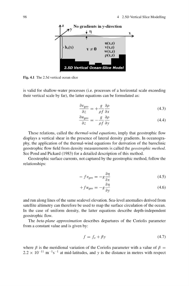
Fig. 4.1 The 2.5d vertical ocean slice
is valid for shallow-water processes (i.e. processes of a horizontal scale exceeding
their vertical scale by far), the latter equations can be formulated as:
∂v geo
∂z
= +
g
ρ f
∂ρ
∂ x
(4.3)
∂u geo
∂z
= −
g
ρ f
∂ρ
∂ y
(4.4)
These relations, called the thermal-wind equations, imply that geostrophic flow
displays a vertical shear in the presence of lateral density gradients. In oceanography, the application of the thermal-wind equations for derivation of the baroclinic
geostrophic flow field from density measurements is called the geostrophic method.
See Pond and Pickard (1983) for a detailed description of this method.
Geostrophic surface currents, not captured by the geostrophic method, follow the
relationships:
− f v geo = −g
∂η
∂ x
(4.5)
+ f u geo = −g
∂η
∂ y
(4.6)
and run along lines of the same sealevel elevation. Sea-level anomalies derived from
satellite altimetry can therefore be used to map the surface circulation of the ocean.
In the case of uniform density, the latter equations describe depth-independent
geostrophic flow.
The beta-plane approximation describes departures of the Coriolis parameter
from a constant value and is given by:
f = f o + βy
(4.7)
where β is the meridional variation of the Coriolis parameter with a value of β =
2.2 × 10
−11 m
−1 s
−1 at mid-latitudes, and y is the distance in metres with respect
4 2.5D Vertical Slice Modelling
Fig. 4.1 The 2.5d vertical ocean slice
is valid for shallow-water processes (i.e. processes of a horizontal scale exceeding
their vertical scale by far), the latter equations can be formulated as:
∂v geo
∂z
= +
g
ρ f
∂ρ
∂ x
(4.3)
∂u geo
∂z
= −
g
ρ f
∂ρ
∂ y
(4.4)
These relations, called the thermal-wind equations, imply that geostrophic flow
displays a vertical shear in the presence of lateral density gradients. In oceanography, the application of the thermal-wind equations for derivation of the baroclinic
geostrophic flow field from density measurements is called the geostrophic method.
See Pond and Pickard (1983) for a detailed description of this method.
Geostrophic surface currents, not captured by the geostrophic method, follow the
relationships:
− f v geo = −g
∂η
∂ x
(4.5)
+ f u geo = −g
∂η
∂ y
(4.6)
and run along lines of the same sealevel elevation. Sea-level anomalies derived from
satellite altimetry can therefore be used to map the surface circulation of the ocean.
In the case of uniform density, the latter equations describe depth-independent
geostrophic flow.
The beta-plane approximation describes departures of the Coriolis parameter
from a constant value and is given by:
f = f o + βy
(4.7)
where β is the meridional variation of the Coriolis parameter with a value of β =
2.2 × 10
−11 m
−1 s
−1 at mid-latitudes, and y is the distance in metres with respect