

3.25 Exercise 15: Inverse Estuaries
95
∂ρ
∂t
=
ρ o β S o + ρ
E
h
(3.93)
In the model, this density change is distributed in the uppermost grid cell (h =
Δz). Convection by unstable density stratification can mix this salinity anomaly
to deeper layers. Owing to coarse grid spacing, convective mixing needs to be
parameterised. This is done here via an increase of eddy diffusivity to a value of
k z = 0.01 m
2
/s. The total simulation time is 20 days. The evaporative forcing is
applied only for the first 10 days and thereafter disabled. Reasons for this treatment
will become obvious with inspection of the results.
3.25.3 Results
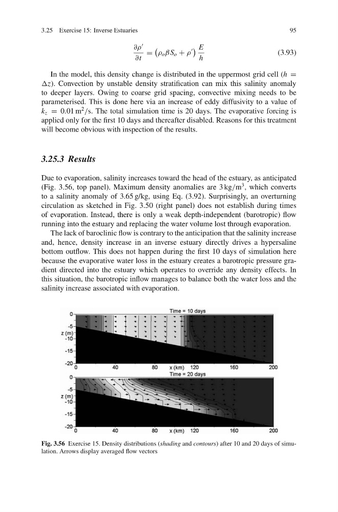
Due to evaporation, salinity increases toward the head of the estuary, as anticipated
(Fig. 3.56, top panel). Maximum density anomalies are 3 kg/m
3 , which converts
to a salinity anomaly of 3.65 g/kg, using Eq. (3.92). Surprisingly, an overturning
circulation as sketched in Fig. 3.50 (right panel) does not establish during times
of evaporation. Instead, there is only a weak depth-independent (barotropic) flow
running into the estuary and replacing the water volume lost through evaporation.
The lack of baroclinic flow is contrary to the anticipation that the salinity increase
and, hence, density increase in an inverse estuary directly drives a hypersaline
bottom outflow. This does not happen during the first 10 days of simulation here
because the evaporative water loss in the estuary creates a barotropic pressure gradient directed into the estuary which operates to override any density effects. In
this situation, the barotropic inflow manages to balance both the water loss and the
salinity increase associated with evaporation.
Fig. 3.56 Exercise 15. Density distributions (shading and contours) after 10 and 20 days of simulation. Arrows display averaged flow vectors
95
∂ρ
∂t
=
ρ o β S o + ρ
E
h
(3.93)
In the model, this density change is distributed in the uppermost grid cell (h =
Δz). Convection by unstable density stratification can mix this salinity anomaly
to deeper layers. Owing to coarse grid spacing, convective mixing needs to be
parameterised. This is done here via an increase of eddy diffusivity to a value of
k z = 0.01 m
2
/s. The total simulation time is 20 days. The evaporative forcing is
applied only for the first 10 days and thereafter disabled. Reasons for this treatment
will become obvious with inspection of the results.
3.25.3 Results
Due to evaporation, salinity increases toward the head of the estuary, as anticipated
(Fig. 3.56, top panel). Maximum density anomalies are 3 kg/m
3 , which converts
to a salinity anomaly of 3.65 g/kg, using Eq. (3.92). Surprisingly, an overturning
circulation as sketched in Fig. 3.50 (right panel) does not establish during times
of evaporation. Instead, there is only a weak depth-independent (barotropic) flow
running into the estuary and replacing the water volume lost through evaporation.
The lack of baroclinic flow is contrary to the anticipation that the salinity increase
and, hence, density increase in an inverse estuary directly drives a hypersaline
bottom outflow. This does not happen during the first 10 days of simulation here
because the evaporative water loss in the estuary creates a barotropic pressure gradient directed into the estuary which operates to override any density effects. In
this situation, the barotropic inflow manages to balance both the water loss and the
salinity increase associated with evaporation.
Fig. 3.56 Exercise 15. Density distributions (shading and contours) after 10 and 20 days of simulation. Arrows display averaged flow vectors