

54
3 Basics of Geophysical Fluid Dynamics
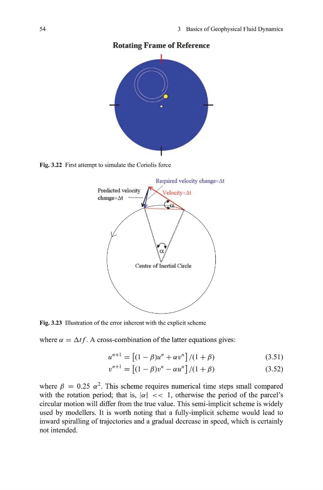
Fig. 3.22 First attempt to simulate the Coriolis force
Fig. 3.23 Illustration of the error inherent with the explicit scheme
where α = Δt f . A cross-combination of the latter equations gives:
u
n+1
=
(1 − β)u
n
+ αv
n
/(1 + β)
(3.51)
v
n+1
=
(1 − β)v
n
− αu
n
/(1 + β)
(3.52)
where β = 0.25 α
2
. This scheme requires numerical time steps small compared
with the rotation period; that is, |α| << 1, otherwise the period of the parcel’s
circular motion will differ from the true value. This semi-implicit scheme is widely
used by modellers. It is worth noting that a fully-implicit scheme would lead to
inward spiralling of trajectories and a gradual decrease in speed, which is certainly
not intended.
3 Basics of Geophysical Fluid Dynamics
Fig. 3.22 First attempt to simulate the Coriolis force
Fig. 3.23 Illustration of the error inherent with the explicit scheme
where α = Δt f . A cross-combination of the latter equations gives:
u
n+1
=
(1 − β)u
n
+ αv
n
/(1 + β)
(3.51)
v
n+1
=
(1 − β)v
n
− αu
n
/(1 + β)
(3.52)
where β = 0.25 α
2
. This scheme requires numerical time steps small compared
with the rotation period; that is, |α| << 1, otherwise the period of the parcel’s
circular motion will differ from the true value. This semi-implicit scheme is widely
used by modellers. It is worth noting that a fully-implicit scheme would lead to
inward spiralling of trajectories and a gradual decrease in speed, which is certainly
not intended.