

48
3 Basics of Geophysical Fluid Dynamics
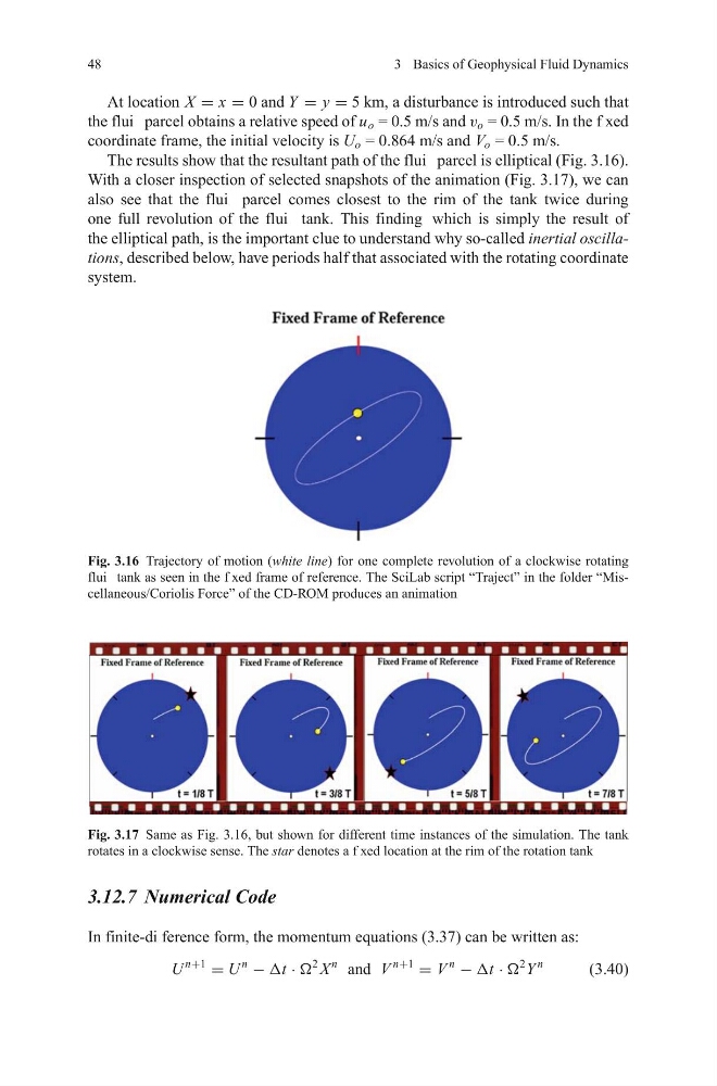
At location X = x = 0 and Y = y = 5 km, a disturbance is introduced such that
the flui parcel obtains a relative speed of u o = 0.5 m/s and v o = 0.5 m/s. In the f xed
coordinate frame, the initial velocity is U o = 0.864 m/s and V o = 0.5 m/s.
The results show that the resultant path of the flui parcel is elliptical (Fig. 3.16).
With a closer inspection of selected snapshots of the animation (Fig. 3.17), we can
also see that the flui parcel comes closest to the rim of the tank twice during
one full revolution of the flui tank. This finding which is simply the result of
the elliptical path, is the important clue to understand why so-called inertial oscillations, described below, have periods half that associated with the rotating coordinate
system.
Fig. 3.16 Trajectory of motion (white line) for one complete revolution of a clockwise rotating
flui tank as seen in the f xed frame of reference. The SciLab script “Traject” in the folder “Miscellaneous/Coriolis Force” of the CD-ROM produces an animation
Fig. 3.17 Same as Fig. 3.16, but shown for different time instances of the simulation. The tank
rotates in a clockwise sense. The star denotes a f xed location at the rim of the rotation tank
3.12.7 Numerical Code
In finite-di ference form, the momentum equations (3.37) can be written as:
U
n+1
= U
n
− Δt · Ω
2
X
n
and V
n+1
= V
n
− Δt · Ω
2
Y
n
(3.40)
3 Basics of Geophysical Fluid Dynamics
At location X = x = 0 and Y = y = 5 km, a disturbance is introduced such that
the flui parcel obtains a relative speed of u o = 0.5 m/s and v o = 0.5 m/s. In the f xed
coordinate frame, the initial velocity is U o = 0.864 m/s and V o = 0.5 m/s.
The results show that the resultant path of the flui parcel is elliptical (Fig. 3.16).
With a closer inspection of selected snapshots of the animation (Fig. 3.17), we can
also see that the flui parcel comes closest to the rim of the tank twice during
one full revolution of the flui tank. This finding which is simply the result of
the elliptical path, is the important clue to understand why so-called inertial oscillations, described below, have periods half that associated with the rotating coordinate
system.
Fig. 3.16 Trajectory of motion (white line) for one complete revolution of a clockwise rotating
flui tank as seen in the f xed frame of reference. The SciLab script “Traject” in the folder “Miscellaneous/Coriolis Force” of the CD-ROM produces an animation
Fig. 3.17 Same as Fig. 3.16, but shown for different time instances of the simulation. The tank
rotates in a clockwise sense. The star denotes a f xed location at the rim of the rotation tank
3.12.7 Numerical Code
In finite-di ference form, the momentum equations (3.37) can be written as:
U
n+1
= U
n
− Δt · Ω
2
X
n
and V
n+1
= V
n
− Δt · Ω
2
Y
n
(3.40)