

40
3 Basics of Geophysical Fluid Dynamics
where the friction coefficien R has units of 1/s. Using an implicit approach for this
term, the finit difference form of this equation reads:
w
n+1
obj − w
n
obj
Δt
= −g
ρ obj − ρ amb
ρ obj
− Rw
n+1
obj
(3.26)
which can be reorganised to yield:
w
n+1
obj =
w
n
obj − Δt · g (ρ obj − ρ amb )/ρ obj
/(1 + RΔt)
(3.27)
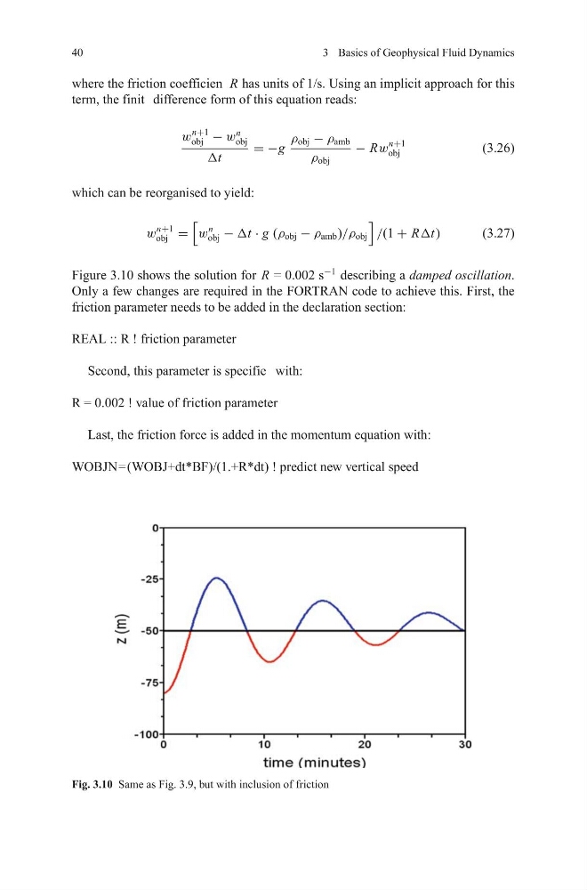
Figure 3.10 shows the solution for R = 0.002 s
−1
describing a damped oscillation.
Only a few changes are required in the FORTRAN code to achieve this. First, the
friction parameter needs to be added in the declaration section:
REAL :: R ! friction parameter
Second, this parameter is specifie with:
R = 0.002 ! value of friction parameter
Last, the friction force is added in the momentum equation with:
WOBJN=(WOBJ+dt*BF)/(1.+R*dt) ! predict new vertical speed
Fig. 3.10 Same as Fig. 3.9, but with inclusion of friction
3 Basics of Geophysical Fluid Dynamics
where the friction coefficien R has units of 1/s. Using an implicit approach for this
term, the finit difference form of this equation reads:
w
n+1
obj − w
n
obj
Δt
= −g
ρ obj − ρ amb
ρ obj
− Rw
n+1
obj
(3.26)
which can be reorganised to yield:
w
n+1
obj =
w
n
obj − Δt · g (ρ obj − ρ amb )/ρ obj
/(1 + RΔt)
(3.27)
Figure 3.10 shows the solution for R = 0.002 s
−1
describing a damped oscillation.
Only a few changes are required in the FORTRAN code to achieve this. First, the
friction parameter needs to be added in the declaration section:
REAL :: R ! friction parameter
Second, this parameter is specifie with:
R = 0.002 ! value of friction parameter
Last, the friction force is added in the momentum equation with:
WOBJN=(WOBJ+dt*BF)/(1.+R*dt) ! predict new vertical speed
Fig. 3.10 Same as Fig. 3.9, but with inclusion of friction