

2.2 First Steps with Finite Differences
9
2.2.4 Implicit Time-Forward Iteration
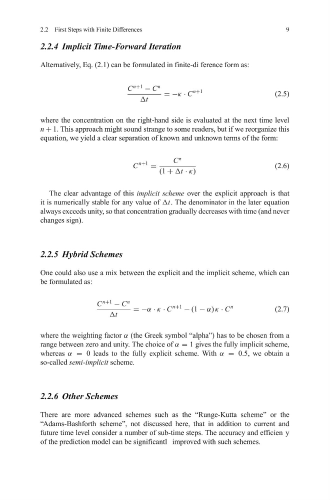
Alternatively, Eq. (2.1) can be formulated in finite-di ference form as:
C
n+1
− C
n
Δt
= −κ · C
n+1
(2.5)
where the concentration on the right-hand side is evaluated at the next time level
n + 1. This approach might sound strange to some readers, but if we reorganize this
equation, we yield a clear separation of known and unknown terms of the form:
C
n+1
=
C
n
(1 + Δt · κ)
(2.6)
The clear advantage of this implicit scheme over the explicit approach is that
it is numerically stable for any value of Δt. The denominator in the later equation
always exceeds unity, so that concentration gradually decreases with time (and never
changes sign).
2.2.5 Hybrid Schemes
One could also use a mix between the explicit and the implicit scheme, which can
be formulated as:
C
n+1
− C
n
Δt
= −α · κ · C
n+1
− (1 − α) κ · C
n
(2.7)
where the weighting factor α (the Greek symbol “alpha”) has to be chosen from a
range between zero and unity. The choice of α = 1 gives the fully implicit scheme,
whereas α = 0 leads to the fully explicit scheme. With α = 0.5, we obtain a
so-called semi-implicit scheme.
2.2.6 Other Schemes
There are more advanced schemes such as the “Runge-Kutta scheme” or the
“Adams-Bashforth scheme”, not discussed here, that in addition to current and
future time level consider a number of sub-time steps. The accuracy and efficien y
of the prediction model can be significantl improved with such schemes.
9
2.2.4 Implicit Time-Forward Iteration
Alternatively, Eq. (2.1) can be formulated in finite-di ference form as:
C
n+1
− C
n
Δt
= −κ · C
n+1
(2.5)
where the concentration on the right-hand side is evaluated at the next time level
n + 1. This approach might sound strange to some readers, but if we reorganize this
equation, we yield a clear separation of known and unknown terms of the form:
C
n+1
=
C
n
(1 + Δt · κ)
(2.6)
The clear advantage of this implicit scheme over the explicit approach is that
it is numerically stable for any value of Δt. The denominator in the later equation
always exceeds unity, so that concentration gradually decreases with time (and never
changes sign).
2.2.5 Hybrid Schemes
One could also use a mix between the explicit and the implicit scheme, which can
be formulated as:
C
n+1
− C
n
Δt
= −α · κ · C
n+1
− (1 − α) κ · C
n
(2.7)
where the weighting factor α (the Greek symbol “alpha”) has to be chosen from a
range between zero and unity. The choice of α = 1 gives the fully implicit scheme,
whereas α = 0 leads to the fully explicit scheme. With α = 0.5, we obtain a
so-called semi-implicit scheme.
2.2.6 Other Schemes
There are more advanced schemes such as the “Runge-Kutta scheme” or the
“Adams-Bashforth scheme”, not discussed here, that in addition to current and
future time level consider a number of sub-time steps. The accuracy and efficien y
of the prediction model can be significantl improved with such schemes.