

2.1 The Decay Problem
7
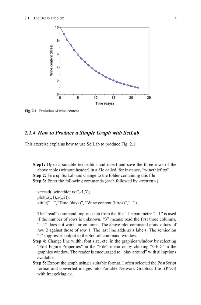
Fig. 2.1 Evolution of wine content
2.1.4 How to Produce a Simple Graph with SciLab
This exercise explains how to use SciLab to produce Fig. 2.1.
Step1: Open a suitable text editor and insert and save the three rows of the
above table (without header) in a f le called, for instance, “winethief.txt”.
Step 2: Fire up SciLab and change to the folder containing this file
Step 3: Enter the following commands (each followed by):
x=read(“winethief.txt”,-1,3);
plot(x(:,1),x(:,2));
xtitle(“ ”,“Time (days)”, “Wine content (litres)”,“ ”)
The “read” command imports data from the file The parameter “−1” is used
if the number of rows is unknown. “3” means: read the f rst three columns,
“−1” does not work for columns. The above plot command plots values of
row 2 against those of row 1. The last line adds axis labels. The semicolon
“;” suppresses output to the SciLab command window.
Step 4: Change line width, font size, etc. in the graphics window by selecting
“Edit Figure Properties” in the “File” menu or by clicking “GED” in the
graphics window. The reader is encouraged to “play around” with all options
available.
Step 5: Export the graph using a suitable format. I often selected the PostScript
format and converted images into Portable Network Graphics file (PNG)
with ImageMagick.
7
Fig. 2.1 Evolution of wine content
2.1.4 How to Produce a Simple Graph with SciLab
This exercise explains how to use SciLab to produce Fig. 2.1.
Step1: Open a suitable text editor and insert and save the three rows of the
above table (without header) in a f le called, for instance, “winethief.txt”.
Step 2: Fire up SciLab and change to the folder containing this file
Step 3: Enter the following commands (each followed by
x=read(“winethief.txt”,-1,3);
plot(x(:,1),x(:,2));
xtitle(“ ”,“Time (days)”, “Wine content (litres)”,“ ”)
The “read” command imports data from the file The parameter “−1” is used
if the number of rows is unknown. “3” means: read the f rst three columns,
“−1” does not work for columns. The above plot command plots values of
row 2 against those of row 1. The last line adds axis labels. The semicolon
“;” suppresses output to the SciLab command window.
Step 4: Change line width, font size, etc. in the graphics window by selecting
“Edit Figure Properties” in the “File” menu or by clicking “GED” in the
graphics window. The reader is encouraged to “play around” with all options
available.
Step 5: Export the graph using a suitable format. I often selected the PostScript
format and converted images into Portable Network Graphics file (PNG)
with ImageMagick.