

6.15 Exercise 21: Frontal Instability
159
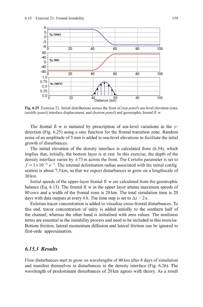
Fig. 6.25 Exercise 21. Initial distributions across the front of (top panel) sea-level elevation (cm),
(middle panel) interface displacement, and (bottom panel) and geostrophic frontal fl w
The frontal fl w is initiated by prescription of sea-level variations in the ydirection (Fig. 6.25) using a sine function for the frontal transition zone. Random
noise of an amplitude of 5 mm is added to sea-level elevations to facilitate the inital
growth of disturbances.
The initial elevation of the density interface is calculated from (6.54), which
implies that, initially, the bottom layer is at rest. In this exercise, the depth of the
density interface varies by ±73 m across the front. The Coriolis parameter is set to
f = 1×10
−4
s
−1
. The internal deformation radius associated with the initial config
uration is about 7.5 km, so that we expect disturbances to grow on a lengthscale of
30 km.
Initial speeds of the upper-layer frontal fl w are calculated from the geostrophic
balance (Eq. 6.13). The frontal fl w in the upper layer attains maximum speeds of
80 cm/s and a width of the frontal zone is 20 km. The total simulation time is 20
days with data outputs at every 6 h. The time step is set to Δt = 2 s.
Eulerian tracer concentration is added to visualise cross-frontal disturbances. To
this end, tracer concentration of unity is added initially to the southern half of
the channel, whereas the other hand is initialised with zero values. The nonlinear
terms are essential in the instability process and need to be included in this exercise.
Bottom friction, lateral momentum diffusion and lateral friction can be ignored to
first-orde approximation.
6.15.3 Results
Flow disturbances start to grow on wavelengths of 40 km after 8 days of simulation
and manifest themselves in disturbances in the density interface (Fig. 6.26). The
wavelength of predominant disturbances of ˜
20 km agrees with theory. As a result
159
Fig. 6.25 Exercise 21. Initial distributions across the front of (top panel) sea-level elevation (cm),
(middle panel) interface displacement, and (bottom panel) and geostrophic frontal fl w
The frontal fl w is initiated by prescription of sea-level variations in the ydirection (Fig. 6.25) using a sine function for the frontal transition zone. Random
noise of an amplitude of 5 mm is added to sea-level elevations to facilitate the inital
growth of disturbances.
The initial elevation of the density interface is calculated from (6.54), which
implies that, initially, the bottom layer is at rest. In this exercise, the depth of the
density interface varies by ±73 m across the front. The Coriolis parameter is set to
f = 1×10
−4
s
−1
. The internal deformation radius associated with the initial config
uration is about 7.5 km, so that we expect disturbances to grow on a lengthscale of
30 km.
Initial speeds of the upper-layer frontal fl w are calculated from the geostrophic
balance (Eq. 6.13). The frontal fl w in the upper layer attains maximum speeds of
80 cm/s and a width of the frontal zone is 20 km. The total simulation time is 20
days with data outputs at every 6 h. The time step is set to Δt = 2 s.
Eulerian tracer concentration is added to visualise cross-frontal disturbances. To
this end, tracer concentration of unity is added initially to the southern half of
the channel, whereas the other hand is initialised with zero values. The nonlinear
terms are essential in the instability process and need to be included in this exercise.
Bottom friction, lateral momentum diffusion and lateral friction can be ignored to
first-orde approximation.
6.15.3 Results
Flow disturbances start to grow on wavelengths of 40 km after 8 days of simulation
and manifest themselves in disturbances in the density interface (Fig. 6.26). The
wavelength of predominant disturbances of ˜
20 km agrees with theory. As a result