

6.7 Exercise 17: Barotropic Instability
135
grid spacings are set to Δx = Δy = 100 m. The time step is Δt = 3 s. Open
boundaries are treated as cyclic boundaries. Total water depth is set to a uniform
value of 10 m. Random disturbances of 0.1 m in amplitude are added to support the
onset of dynamical instabilities.
Wind-stress forcing, lateral momentum diffusion and bottom friction are disabled. The Coriolis parameter is set to a mid-latitude value of f = 1 × 10
−4
s
−1
(northern hemisphere). The model is forced by prescription of an ambient geostrophic lateral shear fl w of a speed of U = ±0.2 m/s with a shear zone of 800 m
in width (see Fig. 6.7).
The barotropic instability mechanism is visualised by addition of Eulerian tracer
concentration to the model domain with values of unity in the northern half of the
channel and zero values in the southern half. The total simulation time is 36 h with
outputs of variables at every 30 min.
6.7.4 Results
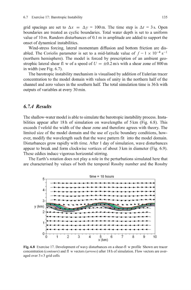
The shallow-water model is able to simulate the barotropic instability process. Instabilities appear after 18 h of simulation on wavelengths of 5 km (Fig. 6.8). This
exceeds f vefold the width of the shear zone and therefore agrees with theory. The
limited size of the model domain and the use of cyclic boundary conditions, however, modify the wavelength such that the wave pattern fit into the model domain.
Disturbances grow rapidly with time. After 1 day of simulation, wave disturbances
appear to break and form clockwise vortices of about 3 km in diameter (Fig. 6.9).
These eddies induce vigorous horizontal stirring.
The Earth’s rotation does not play a role in the perturbations simulated here that
are characterised by values of both the temporal Rossby number and the Rossby
Fig. 6.8 Exercise 17. Development of wavy disturbances on a shear-fl w profile Shown are tracer
concentration (contours) and fl w vectors (arrows) after 18 h of simulation. Flow vectors are averaged over 3×3 grid cells
135
grid spacings are set to Δx = Δy = 100 m. The time step is Δt = 3 s. Open
boundaries are treated as cyclic boundaries. Total water depth is set to a uniform
value of 10 m. Random disturbances of 0.1 m in amplitude are added to support the
onset of dynamical instabilities.
Wind-stress forcing, lateral momentum diffusion and bottom friction are disabled. The Coriolis parameter is set to a mid-latitude value of f = 1 × 10
−4
s
−1
(northern hemisphere). The model is forced by prescription of an ambient geostrophic lateral shear fl w of a speed of U = ±0.2 m/s with a shear zone of 800 m
in width (see Fig. 6.7).
The barotropic instability mechanism is visualised by addition of Eulerian tracer
concentration to the model domain with values of unity in the northern half of the
channel and zero values in the southern half. The total simulation time is 36 h with
outputs of variables at every 30 min.
6.7.4 Results
The shallow-water model is able to simulate the barotropic instability process. Instabilities appear after 18 h of simulation on wavelengths of 5 km (Fig. 6.8). This
exceeds f vefold the width of the shear zone and therefore agrees with theory. The
limited size of the model domain and the use of cyclic boundary conditions, however, modify the wavelength such that the wave pattern fit into the model domain.
Disturbances grow rapidly with time. After 1 day of simulation, wave disturbances
appear to break and form clockwise vortices of about 3 km in diameter (Fig. 6.9).
These eddies induce vigorous horizontal stirring.
The Earth’s rotation does not play a role in the perturbations simulated here that
are characterised by values of both the temporal Rossby number and the Rossby
Fig. 6.8 Exercise 17. Development of wavy disturbances on a shear-fl w profile Shown are tracer
concentration (contours) and fl w vectors (arrows) after 18 h of simulation. Flow vectors are averaged over 3×3 grid cells