

6.5 Exercise 16: Topographic Steering
129
6.5 Exercise 16: Topographic Steering
6.5.1 Aim
The aim of this exercise is to explore the dynamics of barotropic quasi-geostrophic
fl w encountering variable bottom topography.
6.5.2 Model Equations
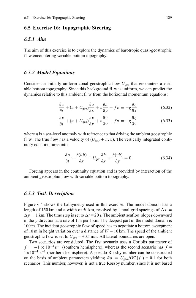
Consider an initially uniform zonal geostrophic f ow U geo that encounters a variable bottom topography. Since this background fl w is uniform, we can predict the
dynamics relative to this ambient fl w from the horizontal momentum equations:
∂u
∂t
+ (u + U geo )
∂u
∂ x
+ v
∂u
∂ y
− f v = −g
∂η
∂ x
(6.32)
∂v
∂t
+ (u + U geo )
∂v
∂ x
+ v
∂v
∂ y
+ f u = −g
∂η
∂ y
(6.33)
where η is a sea-level anomaly with reference to that driving the ambient geostrophic
fl w. The true f ow has a velocity of (U geo + u, v). The vertically integrated continuity equation turns into:
∂η
∂t
+
∂(uh)
∂ x
+ U geo
∂h
∂ x
+
∂(vh)
∂ y
= 0
(6.34)
Forcing appears in the continuity equation and is provided by interaction of the
ambient geostrophic f ow with variable bottom topography.
6.5.3 Task Description
Figure 6.4 shows the bathymetry used in this exercise. The model domain has a
length of 150 km and a width of 50 km, resolved by lateral grid spacings of Δx =
Δy = 1 km. The time step is set to Δt = 20 s. The ambient seafloo slopes downward
in the y direction at a rate of 1 m per 1 km. The deepest part of the model domain is
100 m. The incident geostrophic f ow of speed has to negotiate a bottom escarpment
of 10 m in height variation over a distance of W = 10 km. The speed of the ambient
geostrophic f ow is set to U geo = +0.1 m/s. All lateral boundaries are open.
Two scenarios are considered. The f rst scenario uses a Coriolis parameter of
f = −1 × 10
−4
s
−1
(southern hemisphere), whereas the second scenario has f =
1×10
−4
s
−1
(northern hemisphere). A pseudo Rossby number can be constructed
on the basis of ambient parameters yielding Ro = U geo /(W | f |) = 0.1 for both
scenarios. This number, however, is not a true Rossby number, since it is not based
129
6.5 Exercise 16: Topographic Steering
6.5.1 Aim
The aim of this exercise is to explore the dynamics of barotropic quasi-geostrophic
fl w encountering variable bottom topography.
6.5.2 Model Equations
Consider an initially uniform zonal geostrophic f ow U geo that encounters a variable bottom topography. Since this background fl w is uniform, we can predict the
dynamics relative to this ambient fl w from the horizontal momentum equations:
∂u
∂t
+ (u + U geo )
∂u
∂ x
+ v
∂u
∂ y
− f v = −g
∂η
∂ x
(6.32)
∂v
∂t
+ (u + U geo )
∂v
∂ x
+ v
∂v
∂ y
+ f u = −g
∂η
∂ y
(6.33)
where η is a sea-level anomaly with reference to that driving the ambient geostrophic
fl w. The true f ow has a velocity of (U geo + u, v). The vertically integrated continuity equation turns into:
∂η
∂t
+
∂(uh)
∂ x
+ U geo
∂h
∂ x
+
∂(vh)
∂ y
= 0
(6.34)
Forcing appears in the continuity equation and is provided by interaction of the
ambient geostrophic f ow with variable bottom topography.
6.5.3 Task Description
Figure 6.4 shows the bathymetry used in this exercise. The model domain has a
length of 150 km and a width of 50 km, resolved by lateral grid spacings of Δx =
Δy = 1 km. The time step is set to Δt = 20 s. The ambient seafloo slopes downward
in the y direction at a rate of 1 m per 1 km. The deepest part of the model domain is
100 m. The incident geostrophic f ow of speed has to negotiate a bottom escarpment
of 10 m in height variation over a distance of W = 10 km. The speed of the ambient
geostrophic f ow is set to U geo = +0.1 m/s. All lateral boundaries are open.
Two scenarios are considered. The f rst scenario uses a Coriolis parameter of
f = −1 × 10
−4
s
−1
(southern hemisphere), whereas the second scenario has f =
1×10
−4
s
−1
(northern hemisphere). A pseudo Rossby number can be constructed
on the basis of ambient parameters yielding Ro = U geo /(W | f |) = 0.1 for both
scenarios. This number, however, is not a true Rossby number, since it is not based