

geophysical methods such as seismic refraction, or we must rely on deep-sea
drilling operations or on direct in situ sea floor observations using submersibles or
remote controlled vehicles (ROV). A classic example of stratigraphic sequences of
the outer layers has been extrapolated. This stratigraphy consists of a thin (less
than 2 km thick) basalt-sheeted dyke complex overlying less than 5 km of gabbros
and ultramafic cumulates.
The Summary of Stratigraphic Columns represented on Fig. 4.6 was constructed on the basis of the few available field observations and sampling carried
out by submersible. The geology of these areas will be further described in subsequent chapters dealing with the results obtained in fast spreading ridge segments,
in the Terevaka Transform fault, the Garrett transform in the southeastern Pacific,
the Hess Deep region in the central eastern Pacific, on Mid-Atlantic slow
spreading ridges, the Saint Peter’s and Saint Paul’s Rocks and the Vema fracture
zones in the equatorial Atlantic and northern Atlantic respectively.
The reconstruction of the oceanic stratigraphy is based on the assumption that
the rate of spreading taking place during step faulting remains constant over the
surveyed region (Karson 1998).
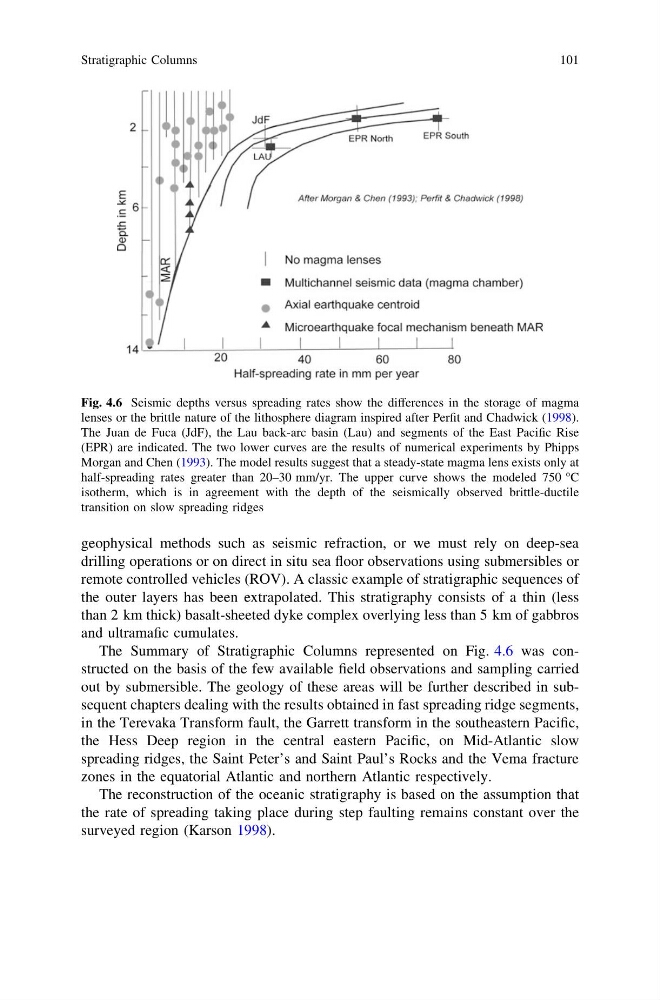
Fig. 4.6 Seismic depths versus spreading rates show the differences in the storage of magma
lenses or the brittle nature of the lithosphere diagram inspired after Perfit and Chadwick (1998).
The Juan de Fuca (JdF), the Lau back-arc basin (Lau) and segments of the East Pacific Rise
(EPR) are indicated. The two lower curves are the results of numerical experiments by Phipps
Morgan and Chen (1993). The model results suggest that a steady-state magma lens exists only at
half-spreading rates greater than 20–30 mm/yr. The upper curve shows the modeled 750 °C
isotherm, which is in agreement with the depth of the seismically observed brittle-ductile
transition on slow spreading ridges
Stratigraphic Columns
101
drilling operations or on direct in situ sea floor observations using submersibles or
remote controlled vehicles (ROV). A classic example of stratigraphic sequences of
the outer layers has been extrapolated. This stratigraphy consists of a thin (less
than 2 km thick) basalt-sheeted dyke complex overlying less than 5 km of gabbros
and ultramafic cumulates.
The Summary of Stratigraphic Columns represented on Fig. 4.6 was constructed on the basis of the few available field observations and sampling carried
out by submersible. The geology of these areas will be further described in subsequent chapters dealing with the results obtained in fast spreading ridge segments,
in the Terevaka Transform fault, the Garrett transform in the southeastern Pacific,
the Hess Deep region in the central eastern Pacific, on Mid-Atlantic slow
spreading ridges, the Saint Peter’s and Saint Paul’s Rocks and the Vema fracture
zones in the equatorial Atlantic and northern Atlantic respectively.
The reconstruction of the oceanic stratigraphy is based on the assumption that
the rate of spreading taking place during step faulting remains constant over the
surveyed region (Karson 1998).
Fig. 4.6 Seismic depths versus spreading rates show the differences in the storage of magma
lenses or the brittle nature of the lithosphere diagram inspired after Perfit and Chadwick (1998).
The Juan de Fuca (JdF), the Lau back-arc basin (Lau) and segments of the East Pacific Rise
(EPR) are indicated. The two lower curves are the results of numerical experiments by Phipps
Morgan and Chen (1993). The model results suggest that a steady-state magma lens exists only at
half-spreading rates greater than 20–30 mm/yr. The upper curve shows the modeled 750 °C
isotherm, which is in agreement with the depth of the seismically observed brittle-ductile
transition on slow spreading ridges
Stratigraphic Columns
101