

17 Some Reflections on Thirty-Five Years of Ocean Color Remote Sensing
293
scattering (L a ) and a component due to the water-leaving radiance (L w ) transmitted
(t) to the top of the atmosphere:
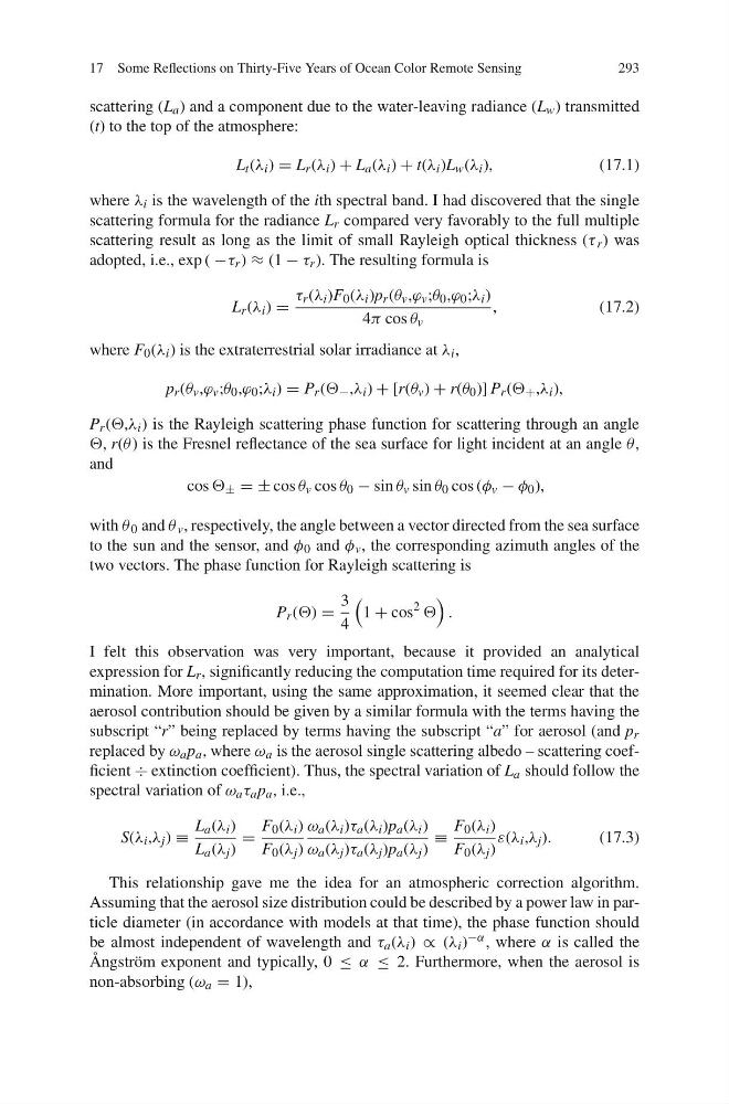
L t (λ i ) = L r (λ i ) + L a (λ i ) + t(λ i )L w (λ i ),
(17.1)
where λ i is the wavelength of the ith spectral band. I had discovered that the single
scattering formula for the radiance L r compared very favorably to the full multiple
scattering result as long as the limit of small Rayleigh optical thickness (τ r ) was
adopted, i.e., exp ( −τ r ) ≈ (1 − τ r ). The resulting formula is
L r (λ i ) =
τ r (λ i )F 0 (λ i )p r (θ v ,ϕ v ;θ 0 ,ϕ 0 ;λ i )
4π cos θ v
,
(17.2)
where F 0 (λ i ) is the extraterrestrial solar irradiance at λ i ,
p r (θ v ,ϕ v ;θ 0 ,ϕ 0 ;λ i ) = P r ( − ,λ i ) + [r(θ v ) + r(θ 0 )] P r ( + ,λ i ),
P r (,λ i ) is the Rayleigh scattering phase function for scattering through an angle
, r(θ ) is the Fresnel reflectance of the sea surface for light incident at an angle θ ,
and
cos ± = ± cos θ v cos θ 0 − sin θ v sin θ 0 cos (φ v − φ 0 ),
with θ 0 and θ v , respectively, the angle between a vector directed from the sea surface
to the sun and the sensor, and φ 0 and φ v , the corresponding azimuth angles of the
two vectors. The phase function for Rayleigh scattering is
P r () =
3
4
1 + cos
2
.
I felt this observation was very important, because it provided an analytical
expression for L r , significantly reducing the computation time required for its determination. More important, using the same approximation, it seemed clear that the
aerosol contribution should be given by a similar formula with the terms having the
subscript “r” being replaced by terms having the subscript “a” for aerosol (and p r
replaced by ω a p a , where ω a is the aerosol single scattering albedo – scattering coefficient ÷ extinction coefficient). Thus, the spectral variation of L a should follow the
spectral variation of ω a τ a p a , i.e.,
S(λ i ,λ j ) ≡
L a (λ i )
L a (λ j )
=
F 0 (λ i )
F 0 (λ j )
ω a (λ i )τ a (λ i )p a (λ i )
ω a (λ j )τ a (λ j )p a (λ j )
≡
F 0 (λ i )
F 0 (λ j )
ε(λ i ,λ j ).
(17.3)
This relationship gave me the idea for an atmospheric correction algorithm.
Assuming that the aerosol size distribution could be described by a power law in particle diameter (in accordance with models at that time), the phase function should
be almost independent of wavelength and τ a (λ i ) ∝ (λ i ) −α , where α is called the
Ångström exponent and typically, 0 ≤ α ≤ 2. Furthermore, when the aerosol is
non-absorbing (ω a = 1),
293
scattering (L a ) and a component due to the water-leaving radiance (L w ) transmitted
(t) to the top of the atmosphere:
L t (λ i ) = L r (λ i ) + L a (λ i ) + t(λ i )L w (λ i ),
(17.1)
where λ i is the wavelength of the ith spectral band. I had discovered that the single
scattering formula for the radiance L r compared very favorably to the full multiple
scattering result as long as the limit of small Rayleigh optical thickness (τ r ) was
adopted, i.e., exp ( −τ r ) ≈ (1 − τ r ). The resulting formula is
L r (λ i ) =
τ r (λ i )F 0 (λ i )p r (θ v ,ϕ v ;θ 0 ,ϕ 0 ;λ i )
4π cos θ v
,
(17.2)
where F 0 (λ i ) is the extraterrestrial solar irradiance at λ i ,
p r (θ v ,ϕ v ;θ 0 ,ϕ 0 ;λ i ) = P r ( − ,λ i ) + [r(θ v ) + r(θ 0 )] P r ( + ,λ i ),
P r (,λ i ) is the Rayleigh scattering phase function for scattering through an angle
, r(θ ) is the Fresnel reflectance of the sea surface for light incident at an angle θ ,
and
cos ± = ± cos θ v cos θ 0 − sin θ v sin θ 0 cos (φ v − φ 0 ),
with θ 0 and θ v , respectively, the angle between a vector directed from the sea surface
to the sun and the sensor, and φ 0 and φ v , the corresponding azimuth angles of the
two vectors. The phase function for Rayleigh scattering is
P r () =
3
4
1 + cos
2
.
I felt this observation was very important, because it provided an analytical
expression for L r , significantly reducing the computation time required for its determination. More important, using the same approximation, it seemed clear that the
aerosol contribution should be given by a similar formula with the terms having the
subscript “r” being replaced by terms having the subscript “a” for aerosol (and p r
replaced by ω a p a , where ω a is the aerosol single scattering albedo – scattering coefficient ÷ extinction coefficient). Thus, the spectral variation of L a should follow the
spectral variation of ω a τ a p a , i.e.,
S(λ i ,λ j ) ≡
L a (λ i )
L a (λ j )
=
F 0 (λ i )
F 0 (λ j )
ω a (λ i )τ a (λ i )p a (λ i )
ω a (λ j )τ a (λ j )p a (λ j )
≡
F 0 (λ i )
F 0 (λ j )
ε(λ i ,λ j ).
(17.3)
This relationship gave me the idea for an atmospheric correction algorithm.
Assuming that the aerosol size distribution could be described by a power law in particle diameter (in accordance with models at that time), the phase function should
be almost independent of wavelength and τ a (λ i ) ∝ (λ i ) −α , where α is called the
Ångström exponent and typically, 0 ≤ α ≤ 2. Furthermore, when the aerosol is
non-absorbing (ω a = 1),