

0
&
~o
:a
E 8 C}I
0
~
8
~
0
.... 8
~ ....
"' E 8 0
....
·
0
8
C?
80
85
90
95
Calendar Year
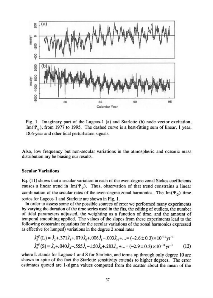
Fig. 1. Imaginary part of the Lageos-1 (a) and Starlette (b) node vector excitation,
Im(\fI Q)' from 1977 to 1995. The dashed curve is a best-fitting sum of linear, 1 year,
18.6-year and other tidal perturbation signals.
Also, low frequency but non-secular variations in the atmospheric and oceanic mass
distribution my be biasing our results.
Secular Variations
Eq. (11) shows that a secular variation in each of the even-degree zonal Stokes coefficients
causes a linear trend in Im(\fI Q)' Thus, observation of that trend constrains a linear
combination of the secular rates of the even-degree zonal harmonics. The Im(\fI Q) time
series for Lageos-1 and Starlette are shown in Fig. 1.
In order to assess some of the possible sources of error we performed many experiments
by varying the duration of the time series used in the fits, the editing of outliers, the number
of tidal parameters adjusted, the weighting as a function of time, and the amount of
temporal smoothing applied. The values of the slopes from these experiments lead to the
following constraint equations for the secular variations of the zonal harmonics expressed
as effective (or lumped) variations in the degree 2 zonal rates
• eff
•
•
•
• •
-11
-1
12 (L) = 12+.37114+.07916+.00618-.003110+"'= (-2.6 ± 0.3) x 10 yr
• eff
_ .
•
• _ .
•
_
-11
-1
12 (S)-1 2 +.0401 4 -.5551 6 .15018+.28311O+ ... -(-2.9±0.3)xlO yr
(12)
where L stands for Lageos-l and S for Starlette, and terms up through only degree 10 are
shown in spite of the fact the Starlette sensitivity extends to higher degrees. The error
estimates quoted are I-sigma values computed from the scatter about the mean of the
37
&
~o
:a
E 8 C}I
0
~
8
~
0
.... 8
~ ....
"' E 8 0
....
·
0
8
C?
80
85
90
95
Calendar Year
Fig. 1. Imaginary part of the Lageos-1 (a) and Starlette (b) node vector excitation,
Im(\fI Q)' from 1977 to 1995. The dashed curve is a best-fitting sum of linear, 1 year,
18.6-year and other tidal perturbation signals.
Also, low frequency but non-secular variations in the atmospheric and oceanic mass
distribution my be biasing our results.
Secular Variations
Eq. (11) shows that a secular variation in each of the even-degree zonal Stokes coefficients
causes a linear trend in Im(\fI Q)' Thus, observation of that trend constrains a linear
combination of the secular rates of the even-degree zonal harmonics. The Im(\fI Q) time
series for Lageos-1 and Starlette are shown in Fig. 1.
In order to assess some of the possible sources of error we performed many experiments
by varying the duration of the time series used in the fits, the editing of outliers, the number
of tidal parameters adjusted, the weighting as a function of time, and the amount of
temporal smoothing applied. The values of the slopes from these experiments lead to the
following constraint equations for the secular variations of the zonal harmonics expressed
as effective (or lumped) variations in the degree 2 zonal rates
• eff
•
•
•
• •
-11
-1
12 (L) = 12+.37114+.07916+.00618-.003110+"'= (-2.6 ± 0.3) x 10 yr
• eff
_ .
•
• _ .
•
_
-11
-1
12 (S)-1 2 +.0401 4 -.5551 6 .15018+.28311O+ ... -(-2.9±0.3)xlO yr
(12)
where L stands for Lageos-l and S for Starlette, and terms up through only degree 10 are
shown in spite of the fact the Starlette sensitivity extends to higher degrees. The error
estimates quoted are I-sigma values computed from the scatter about the mean of the
37