

(11)
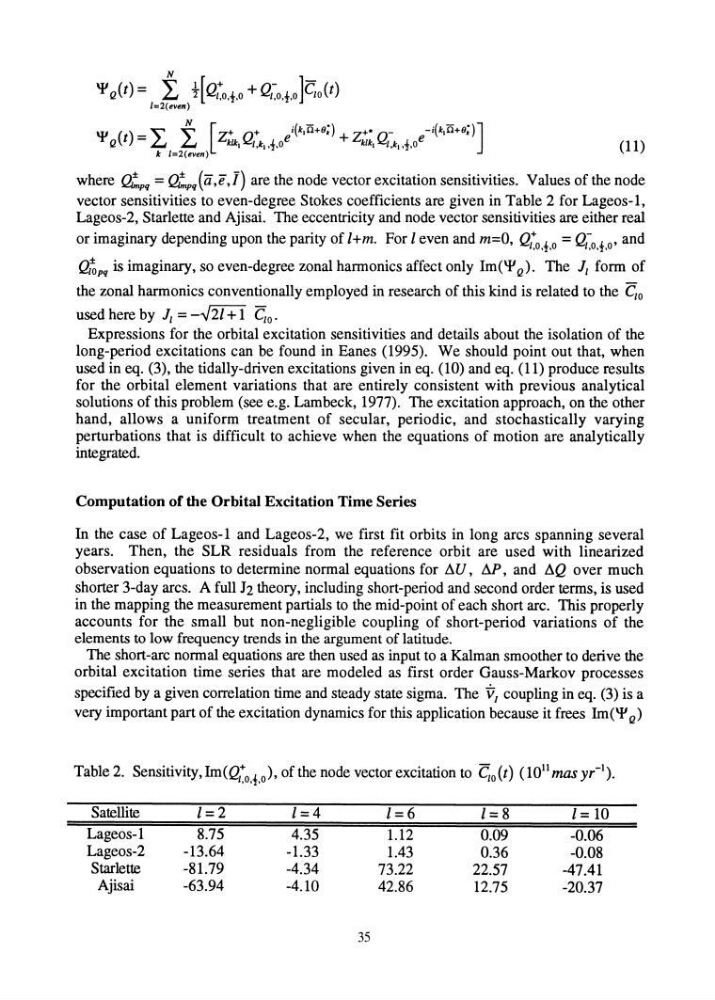
where ~q = Q!pq(a,e,l) are the node vector excitation sensitivities. Values of the node
vector sensitivities to even-degree Stokes coefficients are given in Table 2 for Lageos-l,
Lageos-2, Starlette and Ajisai. The eccentricity and node vector sensitivities are either real
or imaginary depending upon the parity of I+m. For 1 even and m=O, QZo.t. o = Q'~O.t.O' and
Q~pq is imaginary, so even-degree zonal harmonics affect only Im('¥ Q). The J, form of
the zonal harmonics conventionally employed in research of this kind is related to the C/O
used here by J, = -..J21 + 1 C/O.
Expressions for the orbital excitation sensitivities and details about the isolation of the
long-period excitations can be found in Eanes (1995). We should point out that, when
used in eq. (3), the tidally-driven excitations given in eq. (10) and eq. (11) produce results
for the orbital element variations that are entirely consistent with previous analytical
solutions of this problem (see e.g. Lambeck, 1977). The excitation approach, on the other
hand, allows a uniform treatment of secular, periodic, and stochastically varying
perturbations that is difficult to achieve when the equations of motion are analytically
integrated.
Computation of the Orbital Excitation Time Series
In the case of Lageos-l and Lageos-2, we first fit orbits in long arcs spanning several
years. Then, the SLR residuals from the reference orbit are used with linearized
observation equations to determine normal equations for t1U, A.P, and t1Q over much
shorter 3-day arcs. A full 12 theory, including short-period and second order terms, is used
in the mapping the measurement partials to the mid-point of each short arc. This properly
accounts for the small but non-negligible coupling of short-period variations of the
elements to low frequency trends in the argument of latitude.
The short-arc normal equations are then used as input to a Kalman smoother to derive the
orbital excitation time series that are modeled as first order Gauss-Markov processes
specified by a given correlation time and steady state sigma. The VI coupling in eq. (3) is a
very important part of the excitation dynamics for this application because it frees Im('¥ Q)
Table 2. Sensitivity, Im(QZo.t. o ), of the node vector excitation to C/O(t) (1011 mas yr- 1 ).
Satellite
1=2
1=4
1=6
1= 8
1= 10
Lageos-l
8.75
4.35
1.12
0.09
-0.06
Lageos-2
-13.64
-1.33
1.43
0.36
-0.08
Stadette
-81.79
-4.34
73.22
22.57
-47.41
Ajisai
-63.94
-4.10
42.86
12.75
-20.37
35
where ~q = Q!pq(a,e,l) are the node vector excitation sensitivities. Values of the node
vector sensitivities to even-degree Stokes coefficients are given in Table 2 for Lageos-l,
Lageos-2, Starlette and Ajisai. The eccentricity and node vector sensitivities are either real
or imaginary depending upon the parity of I+m. For 1 even and m=O, QZo.t. o = Q'~O.t.O' and
Q~pq is imaginary, so even-degree zonal harmonics affect only Im('¥ Q). The J, form of
the zonal harmonics conventionally employed in research of this kind is related to the C/O
used here by J, = -..J21 + 1 C/O.
Expressions for the orbital excitation sensitivities and details about the isolation of the
long-period excitations can be found in Eanes (1995). We should point out that, when
used in eq. (3), the tidally-driven excitations given in eq. (10) and eq. (11) produce results
for the orbital element variations that are entirely consistent with previous analytical
solutions of this problem (see e.g. Lambeck, 1977). The excitation approach, on the other
hand, allows a uniform treatment of secular, periodic, and stochastically varying
perturbations that is difficult to achieve when the equations of motion are analytically
integrated.
Computation of the Orbital Excitation Time Series
In the case of Lageos-l and Lageos-2, we first fit orbits in long arcs spanning several
years. Then, the SLR residuals from the reference orbit are used with linearized
observation equations to determine normal equations for t1U, A.P, and t1Q over much
shorter 3-day arcs. A full 12 theory, including short-period and second order terms, is used
in the mapping the measurement partials to the mid-point of each short arc. This properly
accounts for the small but non-negligible coupling of short-period variations of the
elements to low frequency trends in the argument of latitude.
The short-arc normal equations are then used as input to a Kalman smoother to derive the
orbital excitation time series that are modeled as first order Gauss-Markov processes
specified by a given correlation time and steady state sigma. The VI coupling in eq. (3) is a
very important part of the excitation dynamics for this application because it frees Im('¥ Q)
Table 2. Sensitivity, Im(QZo.t. o ), of the node vector excitation to C/O(t) (1011 mas yr- 1 ).
Satellite
1=2
1=4
1=6
1= 8
1= 10
Lageos-l
8.75
4.35
1.12
0.09
-0.06
Lageos-2
-13.64
-1.33
1.43
0.36
-0.08
Stadette
-81.79
-4.34
73.22
22.57
-47.41
Ajisai
-63.94
-4.10
42.86
12.75
-20.37
35