

GEOSAT
ERS 1
TOPE X
1600
c;
t,)
.€
~ 400
-8
0
8
-8
0
8
-8
0
8
Latitude (degrees)
Latitude (degrees)
Latitude (degrees)
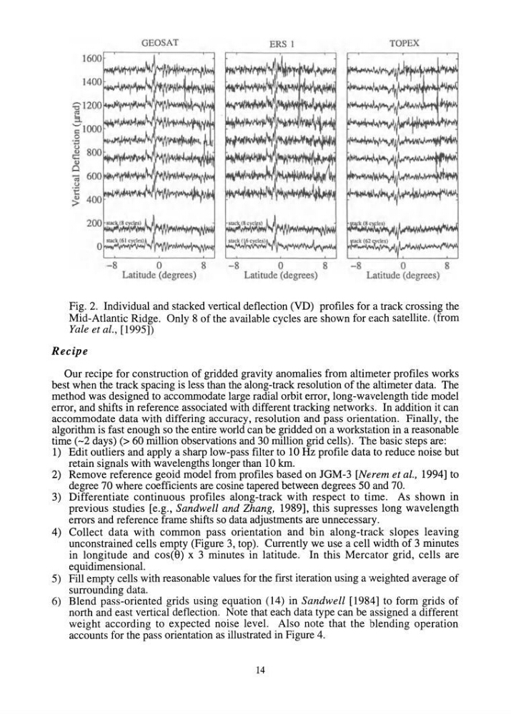
Fig. 2. Individual and stacked vertical deflection (VD) profiles for a track crossing the
Mid-Atlantic Ridge. Only 8 of the available cycles are shown for each satellite. (from
Yale et aI., [1995])
Recipe
Our recipe for construction of gridded gravity anomalies from altimeter profiles works
best when the track spacing is less than the along-track resolution of the altimeter data. The
method was designed to accommodate large radial orbit error, long-wavelength tide model
error, and shifts in reference associated with different tracking networks. In addition it can
accommodate data with differing accuracy, resolution and pass orientation. Finally, the
algorithm is fast enough so the entire world can be gridded on a workstation in a reasonable
time (-2 days) (> 60 million observations and 30 million grid cells). The basic steps are:
1) Edit outliers and apply a sharp low-pass filter to 10 Hz profile data to reduce noise but
retain signals with wavelengths longer than 10 km.
2) Remove reference geoid model from profiles based on JGM-3 [Nerem et aI., 1994] to
degree 70 where coefficients are cosine tapered between degrees 50 and 70.
3) Differentiate continuous profiles along-track with respect to time. As shown in
previous studies [e.g., Sandwell and Zhang, 1989], this supresses long wavelength
errors and reference frame shifts so data adjustments are unnecessary.
4) Collect data with common pass orientation and bin along-track slopes leaving
unconstrained cells empty (Figure 3, top). Currently we use a cell width of 3 minutes
in longitude and cos(S) x 3 minutes in latitude. In this Mercator grid, cells are
equidimensional.
5) Fill empty cells with reasonable values for the first iteration using a weighted average of
surrounding data.
6) Blend pass-oriented grids using equation (14) in Sandwell [1984] to form grids of
north and east vertical deflection. Note that each data type can be assigned a different
weight according to expected noise level. Also note that the blending operation
accounts for the pass orientation as illustrated in Figure 4.
14
ERS 1
TOPE X
1600
c;
t,)
.€
~ 400
-8
0
8
-8
0
8
-8
0
8
Latitude (degrees)
Latitude (degrees)
Latitude (degrees)
Fig. 2. Individual and stacked vertical deflection (VD) profiles for a track crossing the
Mid-Atlantic Ridge. Only 8 of the available cycles are shown for each satellite. (from
Yale et aI., [1995])
Recipe
Our recipe for construction of gridded gravity anomalies from altimeter profiles works
best when the track spacing is less than the along-track resolution of the altimeter data. The
method was designed to accommodate large radial orbit error, long-wavelength tide model
error, and shifts in reference associated with different tracking networks. In addition it can
accommodate data with differing accuracy, resolution and pass orientation. Finally, the
algorithm is fast enough so the entire world can be gridded on a workstation in a reasonable
time (-2 days) (> 60 million observations and 30 million grid cells). The basic steps are:
1) Edit outliers and apply a sharp low-pass filter to 10 Hz profile data to reduce noise but
retain signals with wavelengths longer than 10 km.
2) Remove reference geoid model from profiles based on JGM-3 [Nerem et aI., 1994] to
degree 70 where coefficients are cosine tapered between degrees 50 and 70.
3) Differentiate continuous profiles along-track with respect to time. As shown in
previous studies [e.g., Sandwell and Zhang, 1989], this supresses long wavelength
errors and reference frame shifts so data adjustments are unnecessary.
4) Collect data with common pass orientation and bin along-track slopes leaving
unconstrained cells empty (Figure 3, top). Currently we use a cell width of 3 minutes
in longitude and cos(S) x 3 minutes in latitude. In this Mercator grid, cells are
equidimensional.
5) Fill empty cells with reasonable values for the first iteration using a weighted average of
surrounding data.
6) Blend pass-oriented grids using equation (14) in Sandwell [1984] to form grids of
north and east vertical deflection. Note that each data type can be assigned a different
weight according to expected noise level. Also note that the blending operation
accounts for the pass orientation as illustrated in Figure 4.
14