

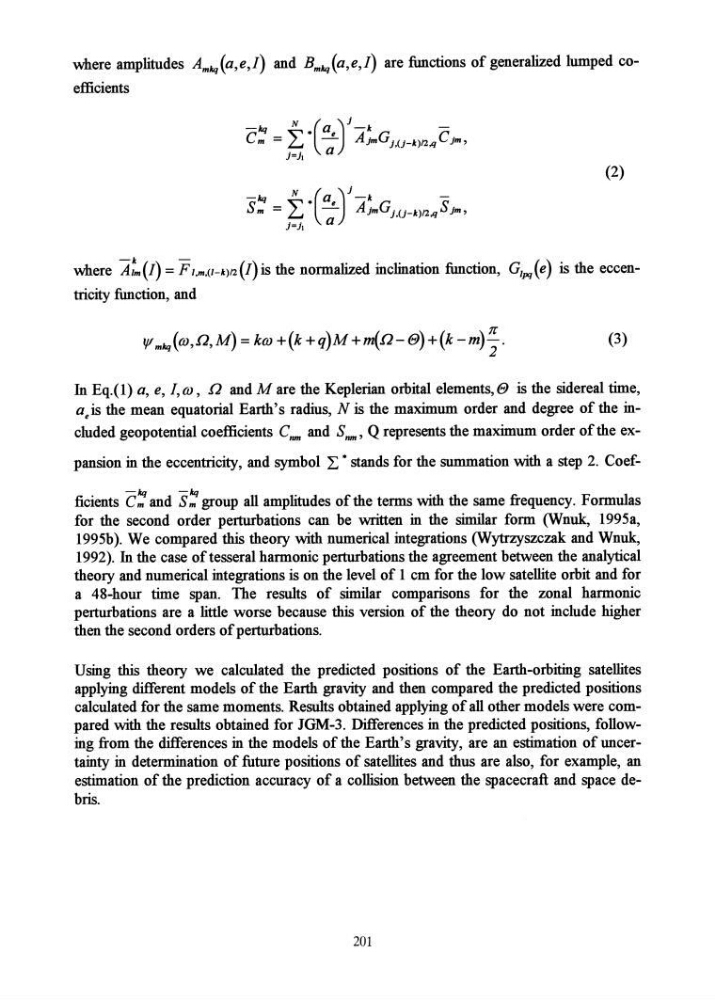
where amplitudes Amkq(a,e,I) and Bmkq(a,e,I) are functions of generalized lumped coefficients
(2)
where A:m(I) = FI,m,(l-k)12 (I) is the normalized inclination function, G1pq(e) is the eccentricity function, and
(3)
In Eq.( 1) a, e, I, OJ, n and M are the Keplerian orbital elements, e is the sidereal time,
aeis the mean equatorial Earth's radius, N is the maximum order and degree of the included geopotential coefficients C nm and Snm' Q represents the maximum order of the expansion in the eccentricity, and symbol ~ * stands for the summation with a step 2. Coefficients C~ and S~ group all amplitudes of the terms with the same frequency. Formulas
for the second order perturbations can be written in the similar form (Wnuk, 1995a,
1995b). We compared this theory with numerical integrations (Wytrzyszczak and Wnuk,
1992). In the case of tesseral harmonic perturbations the agreement between the analytical
theory and numerical integrations is on the level of 1 cm for the low satellite orbit and for
a 48-hour time span. The results of similar comparisons for the zonal harmonic
perturbations are a little worse because this version of the theory do not include higher
then the second orders of perturbations.
Using this theory we calculated the predicted positions of the Earth-orbiting satellites
applying different models of the Earth gravity and then compared the predicted positions
calculated for the same moments. Results obtained applying of all other models were compared with the results obtained for JGM-3. Differences in the predicted positions, following from the differences in the models of the Earth's gravity, are an estimation ofuncertainty in determination of future positions of satellites and thus are also, for example, an
estimation of the prediction accuracy of a collision between the spacecraft and space debris.
201
(2)
where A:m(I) = FI,m,(l-k)12 (I) is the normalized inclination function, G1pq(e) is the eccentricity function, and
(3)
In Eq.( 1) a, e, I, OJ, n and M are the Keplerian orbital elements, e is the sidereal time,
aeis the mean equatorial Earth's radius, N is the maximum order and degree of the included geopotential coefficients C nm and Snm' Q represents the maximum order of the expansion in the eccentricity, and symbol ~ * stands for the summation with a step 2. Coefficients C~ and S~ group all amplitudes of the terms with the same frequency. Formulas
for the second order perturbations can be written in the similar form (Wnuk, 1995a,
1995b). We compared this theory with numerical integrations (Wytrzyszczak and Wnuk,
1992). In the case of tesseral harmonic perturbations the agreement between the analytical
theory and numerical integrations is on the level of 1 cm for the low satellite orbit and for
a 48-hour time span. The results of similar comparisons for the zonal harmonic
perturbations are a little worse because this version of the theory do not include higher
then the second orders of perturbations.
Using this theory we calculated the predicted positions of the Earth-orbiting satellites
applying different models of the Earth gravity and then compared the predicted positions
calculated for the same moments. Results obtained applying of all other models were compared with the results obtained for JGM-3. Differences in the predicted positions, following from the differences in the models of the Earth's gravity, are an estimation ofuncertainty in determination of future positions of satellites and thus are also, for example, an
estimation of the prediction accuracy of a collision between the spacecraft and space debris.
201