

geological and archaeological data from coastal areas or as
a reference surface for evaluating tectonic rates of vertical
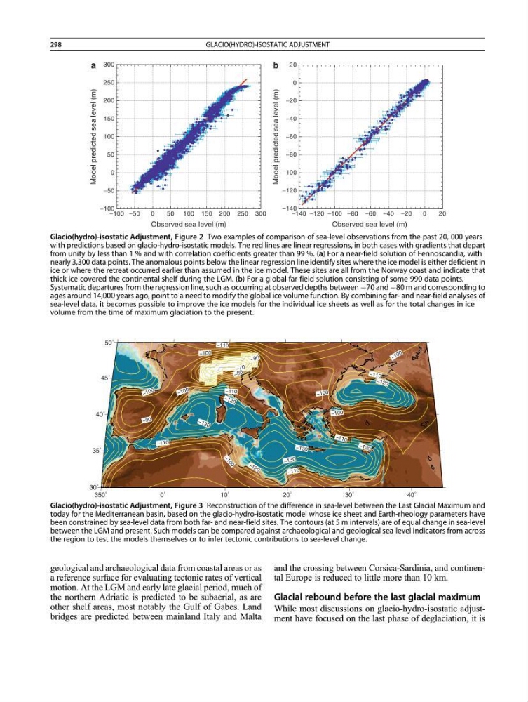
motion. At the LGM and early late glacial period, much of
the northern Adriatic is predicted to be subaerial, as are
other shelf areas, most notably the Gulf of Gabes. Land
bridges are predicted between mainland Italy and Malta
and the crossing between Corsica-Sardinia, and continental Europe is reduced to little more than 10 km.
Glacial rebound before the last glacial maximum
While most discussions on glacio-hydro-isostatic adjustment have focused on the last phase of deglaciation, it is
1 3 0
13 0
13 0
12 0
1 2 0
1 2 0
1 2 0
110
11 0
110
1 1 0
11 0
110
1
0
0
100
1 0 0
100
1 0 0
1 0 0
10 0
90
90
8 0
70
1 3 0
13 0
13 0
12 0
1 2 0
1 2 0
1 2 0
110
11 0
110
1 1 0
11 0
110
1
0
0
100
1 0 0
100
1 0 0
1 0 0
10 0
90
90
8 0
70
Glacio(hydro)-isostatic Adjustment, Figure 3 Reconstruction of the difference in sea-level between the Last Glacial Maximum and
today for the Mediterranean basin, based on the glacio-hydro-isostatic model whose ice sheet and Earth-rheology parameters have
been constrained by sea-level data from both far- and near-field sites. The contours (at 5 m intervals) are of equal change in sea-level
between the LGM and present. Such models can be compared against archaeological and geological sea-level indicators from across
the region to test the models themselves or to infer tectonic contributions to sea-level change.
−100
−50
0
50
100
150
200
250
300
−100 −50
0
50 100 150 200 250 300
Model predicted sea level (m)
−140
−120
−100
−80
−60
−40
−20
0
20
−140 −120 −100 −80 −60 −40 −20
0
20
Model predicted sea level (m)
Observed sea level (m)
Observed sea level (m)
a
b
Glacio(hydro)-isostatic Adjustment, Figure 2 Two examples of comparison of sea-level observations from the past 20, 000 years
with predictions based on glacio-hydro-isostatic models. The red lines are linear regressions, in both cases with gradients that depart
from unity by less than 1 % and with correlation coefficients greater than 99 %. (a) For a near-field solution of Fennoscandia, with
nearly 3,300 data points. The anomalous points below the linear regression line identify sites where the ice model is either deficient in
ice or where the retreat occurred earlier than assumed in the ice model. These sites are all from the Norway coast and indicate that
thick ice covered the continental shelf during the LGM. (b) For a global far-field solution consisting of some 990 data points.
Systematic departures from the regression line, such as occurring at observed depths between À70 and À80 m and corresponding to
ages around 14,000 years ago, point to a need to modify the global ice volume function. By combining far- and near-field analyses of
sea-level data, it becomes possible to improve the ice models for the individual ice sheets as well as for the total changes in ice
volume from the time of maximum glaciation to the present.
298
GLACIO(HYDRO)-ISOSTATIC ADJUSTMENT
a reference surface for evaluating tectonic rates of vertical
motion. At the LGM and early late glacial period, much of
the northern Adriatic is predicted to be subaerial, as are
other shelf areas, most notably the Gulf of Gabes. Land
bridges are predicted between mainland Italy and Malta
and the crossing between Corsica-Sardinia, and continental Europe is reduced to little more than 10 km.
Glacial rebound before the last glacial maximum
While most discussions on glacio-hydro-isostatic adjustment have focused on the last phase of deglaciation, it is
1 3 0
13 0
13 0
12 0
1 2 0
1 2 0
1 2 0
110
11 0
110
1 1 0
11 0
110
1
0
0
100
1 0 0
100
1 0 0
1 0 0
10 0
90
90
8 0
70
1 3 0
13 0
13 0
12 0
1 2 0
1 2 0
1 2 0
110
11 0
110
1 1 0
11 0
110
1
0
0
100
1 0 0
100
1 0 0
1 0 0
10 0
90
90
8 0
70
Glacio(hydro)-isostatic Adjustment, Figure 3 Reconstruction of the difference in sea-level between the Last Glacial Maximum and
today for the Mediterranean basin, based on the glacio-hydro-isostatic model whose ice sheet and Earth-rheology parameters have
been constrained by sea-level data from both far- and near-field sites. The contours (at 5 m intervals) are of equal change in sea-level
between the LGM and present. Such models can be compared against archaeological and geological sea-level indicators from across
the region to test the models themselves or to infer tectonic contributions to sea-level change.
−100
−50
0
50
100
150
200
250
300
−100 −50
0
50 100 150 200 250 300
Model predicted sea level (m)
−140
−120
−100
−80
−60
−40
−20
0
20
−140 −120 −100 −80 −60 −40 −20
0
20
Model predicted sea level (m)
Observed sea level (m)
Observed sea level (m)
a
b
Glacio(hydro)-isostatic Adjustment, Figure 2 Two examples of comparison of sea-level observations from the past 20, 000 years
with predictions based on glacio-hydro-isostatic models. The red lines are linear regressions, in both cases with gradients that depart
from unity by less than 1 % and with correlation coefficients greater than 99 %. (a) For a near-field solution of Fennoscandia, with
nearly 3,300 data points. The anomalous points below the linear regression line identify sites where the ice model is either deficient in
ice or where the retreat occurred earlier than assumed in the ice model. These sites are all from the Norway coast and indicate that
thick ice covered the continental shelf during the LGM. (b) For a global far-field solution consisting of some 990 data points.
Systematic departures from the regression line, such as occurring at observed depths between À70 and À80 m and corresponding to
ages around 14,000 years ago, point to a need to modify the global ice volume function. By combining far- and near-field analyses of
sea-level data, it becomes possible to improve the ice models for the individual ice sheets as well as for the total changes in ice
volume from the time of maximum glaciation to the present.
298
GLACIO(HYDRO)-ISOSTATIC ADJUSTMENT