

64
R.H. Chartier and Chr. P. De Meyer
NI0
0
QI
M,.Q
!ws=0.2
\.
02
0.3
0.4
0.5
6
v
C a
---a~
using constant E t (e~ :6)
~
using parabolic ~t
--e
using linear
C t (~z: 3)
....
using parabolic-constant
(26
(27
C~
09
~0
~t
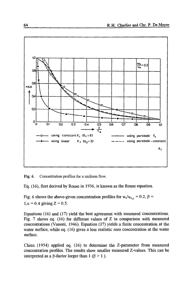
Fig. 6. Concentration profiles for a uniform flow.
Eq. (16), first derived by Rouse in 1936, is known as the Rouse equation.
Fig. 6 shows the above-given concentration profiles for wJu.,~ = 0.2, I~ =
I,K = 0.4 giving Z = 0.5.
Equations (16) and (17) yield the best agreement with measured concentrations.
Fig. 7 shows eq. (16) for different values of Z in comparison with measured
concentrations (Vanoni, 1946). Equation (17) yields a finite concentration at the
water surface, while eq. (16) gives a less realistic zero concentration at the water
surface.
Chien (1954) applied eq. (16) to determine the Z-parameter from measured
concentration profiles. The results show smaller measured Z-values. This can be
interpreted as a 13-factor larger than 1 (13 > 1 ).
R.H. Chartier and Chr. P. De Meyer
NI0
0
QI
M,.Q
!ws=0.2
\.
02
0.3
0.4
0.5
6
v
C a
---a~
using constant E t (e~ :6)
~
using parabolic ~t
--e
using linear
C t (~z: 3)
....
using parabolic-constant
(26
(27
C~
09
~0
~t
Fig. 6. Concentration profiles for a uniform flow.
Eq. (16), first derived by Rouse in 1936, is known as the Rouse equation.
Fig. 6 shows the above-given concentration profiles for wJu.,~ = 0.2, I~ =
I,K = 0.4 giving Z = 0.5.
Equations (16) and (17) yield the best agreement with measured concentrations.
Fig. 7 shows eq. (16) for different values of Z in comparison with measured
concentrations (Vanoni, 1946). Equation (17) yields a finite concentration at the
water surface, while eq. (16) gives a less realistic zero concentration at the water
surface.
Chien (1954) applied eq. (16) to determine the Z-parameter from measured
concentration profiles. The results show smaller measured Z-values. This can be
interpreted as a 13-factor larger than 1 (13 > 1 ).