

132
R.H. Chaflier and Chro P:De Meyer
n
0
1
2
3
R-1
R
,, ~
." X - axis
S O 10)
"~
So (R)
~ItY - axis
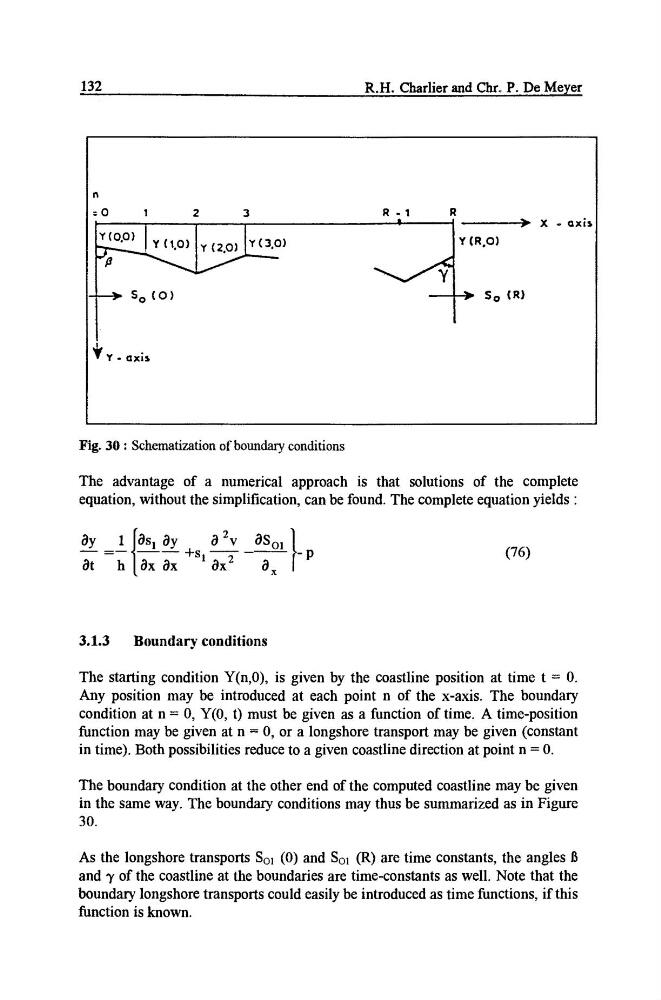
Fig. 30 : Schematization of boundary conditions
The advantage of a numerical approach is that solutions of the complete
equation, without the simplification, can be found. The complete equation yields :
Oy0t -hllOslOY[oxox
O2v OS°l}
]--2---2--- +s I
-p
(76)
Ox 2
O x
3.1.3
Boundary conditions
The starting condition Y(n,0), is given by the coastline position at time t = 0.
Any position may be introduced at each point n of the x-axis. The boundary
condition at n = 0, Y(0, t) must be given as a function of time. A time-position
function may be given at n = 0, or a longshore transport may be given (constant
in time). Both possibilities reduce to a given coastline direction at point n = 0.
The boundary condition at the other end of the computed coastline may be given
in the same way. The boundary conditions may thus be summarized as in Figure
30.
As the longshore transports Sol (0) and So~ (R) are time constants, the angles B
and 7 of the coastline at the boundaries are time-constants as well. Note that the
boundary longshore transports could easily be introduced as time functions, if this
function is known.
R.H. Chaflier and Chro P:De Meyer
n
0
1
2
3
R-1
R
,, ~
." X - axis
S O 10)
"~
So (R)
~ItY - axis
Fig. 30 : Schematization of boundary conditions
The advantage of a numerical approach is that solutions of the complete
equation, without the simplification, can be found. The complete equation yields :
Oy0t -hllOslOY[oxox
O2v OS°l}
]--2---2--- +s I
-p
(76)
Ox 2
O x
3.1.3
Boundary conditions
The starting condition Y(n,0), is given by the coastline position at time t = 0.
Any position may be introduced at each point n of the x-axis. The boundary
condition at n = 0, Y(0, t) must be given as a function of time. A time-position
function may be given at n = 0, or a longshore transport may be given (constant
in time). Both possibilities reduce to a given coastline direction at point n = 0.
The boundary condition at the other end of the computed coastline may be given
in the same way. The boundary conditions may thus be summarized as in Figure
30.
As the longshore transports Sol (0) and So~ (R) are time constants, the angles B
and 7 of the coastline at the boundaries are time-constants as well. Note that the
boundary longshore transports could easily be introduced as time functions, if this
function is known.