

11 Applications of an Oil Drift and Fate Model for Fairway Design
391
cost functions is problematic because of the different nature of the two parameters.
The process of risk minimization tends to connect local minima and to produce meandering tracks, whereas path length minimization tends to generate straight lines.
A reduction of the problem to one single meaningful optimum cost function that
combines the two characteristics is usually not possible. For that reason, a sequential Monte Carlo approach is used, where the first priority is to minimize the cost
function and the path length minimization is of secondary order. During such a process the risk factors and the pathway length need not be weighted against each other
within one optimization cycle.
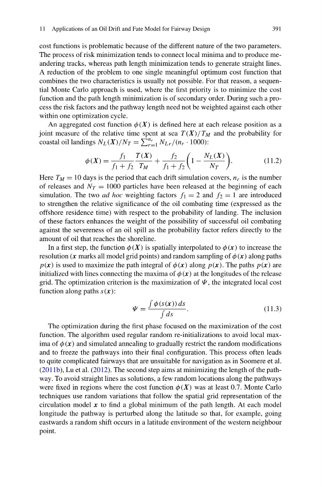
An aggregated cost function φ(X) is defined here at each release position as a
joint measure of the relative time spent at sea T (X)/T M and the probability for
coastal oil landings N L (X)/N T =
n r
r=1 N Lr /(n r · 1000):
φ(X) =
f 1
f 1 + f 2
T (X)
T M
+
f 2
f 1 + f 2
1 −
N L (X)
N T
.
(11.2)
Here T M = 10 days is the period that each drift simulation covers, n r is the number
of releases and N T = 1000 particles have been released at the beginning of each
simulation. The two ad hoc weighting factors f 1 = 2 and f 2 = 1 are introduced
to strengthen the relative significance of the oil combating time (expressed as the
offshore residence time) with respect to the probability of landing. The inclusion
of these factors enhances the weight of the possibility of successful oil combating
against the severeness of an oil spill as the probability factor refers directly to the
amount of oil that reaches the shoreline.
In a first step, the function φ(X) is spatially interpolated to φ(x) to increase the
resolution (x marks all model grid points) and random sampling of φ(x) along paths
p(x) is used to maximize the path integral of φ(x) along p(x). The paths p(x) are
initialized with lines connecting the maxima of φ(x) at the longitudes of the release
grid. The optimization criterion is the maximization of Ψ , the integrated local cost
function along paths s(x):
Ψ =
φ(s(x)) ds
ds
.
(11.3)
The optimization during the first phase focused on the maximization of the cost
function. The algorithm used regular random re-initializations to avoid local maxima of φ(x) and simulated annealing to gradually restrict the random modifications
and to freeze the pathways into their final configuration. This process often leads
to quite complicated fairways that are unsuitable for navigation as in Soomere et al.
(2011b), Lu et al. (2012). The second step aims at minimizing the length of the pathway. To avoid straight lines as solutions, a few random locations along the pathways
were fixed in regions where the cost function φ(X) was at least 0.7. Monte Carlo
techniques use random variations that follow the spatial grid representation of the
circulation model x to find a global minimum of the path length. At each model
longitude the pathway is perturbed along the latitude so that, for example, going
eastwards a random shift occurs in a latitude environment of the western neighbour
point.
391
cost functions is problematic because of the different nature of the two parameters.
The process of risk minimization tends to connect local minima and to produce meandering tracks, whereas path length minimization tends to generate straight lines.
A reduction of the problem to one single meaningful optimum cost function that
combines the two characteristics is usually not possible. For that reason, a sequential Monte Carlo approach is used, where the first priority is to minimize the cost
function and the path length minimization is of secondary order. During such a process the risk factors and the pathway length need not be weighted against each other
within one optimization cycle.
An aggregated cost function φ(X) is defined here at each release position as a
joint measure of the relative time spent at sea T (X)/T M and the probability for
coastal oil landings N L (X)/N T =
n r
r=1 N Lr /(n r · 1000):
φ(X) =
f 1
f 1 + f 2
T (X)
T M
+
f 2
f 1 + f 2
1 −
N L (X)
N T
.
(11.2)
Here T M = 10 days is the period that each drift simulation covers, n r is the number
of releases and N T = 1000 particles have been released at the beginning of each
simulation. The two ad hoc weighting factors f 1 = 2 and f 2 = 1 are introduced
to strengthen the relative significance of the oil combating time (expressed as the
offshore residence time) with respect to the probability of landing. The inclusion
of these factors enhances the weight of the possibility of successful oil combating
against the severeness of an oil spill as the probability factor refers directly to the
amount of oil that reaches the shoreline.
In a first step, the function φ(X) is spatially interpolated to φ(x) to increase the
resolution (x marks all model grid points) and random sampling of φ(x) along paths
p(x) is used to maximize the path integral of φ(x) along p(x). The paths p(x) are
initialized with lines connecting the maxima of φ(x) at the longitudes of the release
grid. The optimization criterion is the maximization of Ψ , the integrated local cost
function along paths s(x):
Ψ =
φ(s(x)) ds
ds
.
(11.3)
The optimization during the first phase focused on the maximization of the cost
function. The algorithm used regular random re-initializations to avoid local maxima of φ(x) and simulated annealing to gradually restrict the random modifications
and to freeze the pathways into their final configuration. This process often leads
to quite complicated fairways that are unsuitable for navigation as in Soomere et al.
(2011b), Lu et al. (2012). The second step aims at minimizing the length of the pathway. To avoid straight lines as solutions, a few random locations along the pathways
were fixed in regions where the cost function φ(X) was at least 0.7. Monte Carlo
techniques use random variations that follow the spatial grid representation of the
circulation model x to find a global minimum of the path length. At each model
longitude the pathway is perturbed along the latitude so that, for example, going
eastwards a random shift occurs in a latitude environment of the western neighbour
point.