

344
T. Soomere
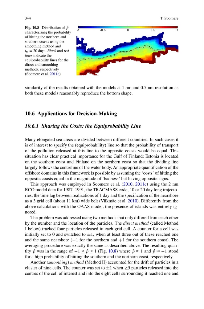
Fig. 10.8 Distribution of ˆ
p
characterizing the probability
of hitting the northern and
southern coasts using the
smoothing method and
t w = 20 days. Black and red
lines indicate the
equiprobability lines for the
direct and smoothing
methods, respectively
(Soomere et al. 2011c)
similarity of the results obtained with the models at 1 nm and 0.5 nm resolution as
both these models reasonably reproduce the bottom shape.
10.6 Applications for Decision-Making
10.6.1 Sharing the Costs: the Equiprobability Line
Many elongated sea areas are divided between different countries. In such cases it
is of interest to specify the (equiprobability) line so that the probability of transport
of the pollution released at this line to the opposite coasts would be equal. This
situation has clear practical importance for the Gulf of Finland: Estonia is located
on the southern coast and Finland on the northern coast so that the dividing line
largely follows the centreline of the water body. An appropriate quantification of the
offshore domains in this framework is possible by assuming the ‘costs’ of hitting the
opposite coasts equal in the magnitude of ‘badness’ but having opposite signs.
This approach was employed in Soomere et al. (2010, 2011c) using the 2 nm
RCO model data for 1987–1991, the TRACMASS code, 10 or 20 day long trajectories, the time lag between realizations of 1 day and the specification of the nearshore
as a 3 grid cell (about 11 km) wide belt (Viikmäe et al. 2010). Differently from the
above calculations with the OAAS model, the presence of islands was entirely ignored.
The problem was addressed using two methods that only differed from each other
by the number and the location of the particles. The direct method (called Method
I below) tracked four particles released in each grid cell. A counter for a cell was
initially set to 0 and switched to ±1, when at least three out of these reached one
and the same nearshore (−1 for the northern and +1 for the southern coast). The
averaging procedure was exactly the same as described above. The resulting quantity ˆ
p was in the range of −1 ≤ ˆ
p ≤ 1 (Fig. 10.8) where ˆ
p ≈ 1 and ˆ
p ≈ −1 stood
for a high probability of hitting the southern and the northern coast, respectively.
Another (smoothing) method (Method II) accounted for the drift of particles in a
cluster of nine cells. The counter was set to ±1 when ≥5 particles released into the
centres of the cell of interest and into the eight cells surrounding it reached one and
T. Soomere
Fig. 10.8 Distribution of ˆ
p
characterizing the probability
of hitting the northern and
southern coasts using the
smoothing method and
t w = 20 days. Black and red
lines indicate the
equiprobability lines for the
direct and smoothing
methods, respectively
(Soomere et al. 2011c)
similarity of the results obtained with the models at 1 nm and 0.5 nm resolution as
both these models reasonably reproduce the bottom shape.
10.6 Applications for Decision-Making
10.6.1 Sharing the Costs: the Equiprobability Line
Many elongated sea areas are divided between different countries. In such cases it
is of interest to specify the (equiprobability) line so that the probability of transport
of the pollution released at this line to the opposite coasts would be equal. This
situation has clear practical importance for the Gulf of Finland: Estonia is located
on the southern coast and Finland on the northern coast so that the dividing line
largely follows the centreline of the water body. An appropriate quantification of the
offshore domains in this framework is possible by assuming the ‘costs’ of hitting the
opposite coasts equal in the magnitude of ‘badness’ but having opposite signs.
This approach was employed in Soomere et al. (2010, 2011c) using the 2 nm
RCO model data for 1987–1991, the TRACMASS code, 10 or 20 day long trajectories, the time lag between realizations of 1 day and the specification of the nearshore
as a 3 grid cell (about 11 km) wide belt (Viikmäe et al. 2010). Differently from the
above calculations with the OAAS model, the presence of islands was entirely ignored.
The problem was addressed using two methods that only differed from each other
by the number and the location of the particles. The direct method (called Method
I below) tracked four particles released in each grid cell. A counter for a cell was
initially set to 0 and switched to ±1, when at least three out of these reached one
and the same nearshore (−1 for the northern and +1 for the southern coast). The
averaging procedure was exactly the same as described above. The resulting quantity ˆ
p was in the range of −1 ≤ ˆ
p ≤ 1 (Fig. 10.8) where ˆ
p ≈ 1 and ˆ
p ≈ −1 stood
for a high probability of hitting the southern and the northern coast, respectively.
Another (smoothing) method (Method II) accounted for the drift of particles in a
cluster of nine cells. The counter was set to ±1 when ≥5 particles released into the
centres of the cell of interest and into the eight cells surrounding it reached one and