

10 Applications of the Inverse Problem of Pollution Propagation
333
conditions the aggregated impact of small-scale features of the motions generally
tends to spread closely packed particles (Richardson 1926; Ollitrault et al. 2005).
It is well known that the spreading of the resulting trajectories in studies based on
this version of TRACMASS has been usually much smaller than the spreading of
real drifters (Jönsson et al. 2004; Engqvist et al. 2006; Döös and Engqvist 2007;
Döös et al. 2008). An implicit consequence from the lack of spreading is that the
nearshore had to be defined as a 3 grid cells wide zone near the coast when the
TRACMASS code was used for the Gulf of Finland (Viikmäe et al. 2010).
10.4.5 Trajectory Simulations in the OAAS Model
The estimates for the spreading of real drifters in the Gulf of Finland (Soomere
et al. 2011e, see also Chap. 8) show that it takes, on average, about 4 days for
two initially closely located particles to drift into different grid cells of the 2 nm
RCO model. This suggests that ignoring sub-grid scale processes may modify a
part of the trajectories but their majority will remain at a distance of less than one
grid step from their actual position. It is natural to assume that further spreading
of the trajectories will mostly occur due to the gradients in the simulated velocity
fields. It is also reasonable to suppose that for the particular horizontal resolution and
length of trajectories, ignoring the subgrid spreading does not significantly affect the
resulting 2D fields and might even suppress the noise in these fields compared to
artificial reproduction of the spreading. Doing so is, however, a major simplification
that might not be entirely justified (Andrejev et al. 2011).
The trajectories were simulated ‘on-line’ (simultaneously with the integration of
the model, see Chap. 7) in runs of the OAAS model (Andrejev et al. 2010, 2011;
Soomere et al. 2011a, 2011b). The scheme accounted for the effect of subgrid-scale
motions. Note again that the exact motions of the particles cannot be restored and the
major benefit from such efforts is that the statistics of spreading (e.g., the absolute
dispersion or the net distance covered by a particle over some time) is represented
more adequately.
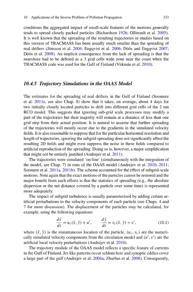
The impact of subgrid turbulence is usually parameterized by adding certain artificial perturbations to the velocity components of each particle (see Chaps. 4 and
7 for more discussion). The displacement of the particles may be calculated, for
example, using the following equations:
d ˜
x
dt
= u c ( ˜
x, ˜
y) + u
,
d ˜
y
dt
= v c ( ˜
x, ˜
y) + v
,
(10.1)
where ( ˜
x, ˜
y) is the instantaneous location of the particle, (u c , v c ) are the numerically simulated velocity components from the circulation model and (u , v ) are the
artificial local velocity perturbations (Andrejev et al. 2010).
The trajectory module of the OAAS model reflects a specific feature of currents
in the Gulf of Finland. Jet-like patterns occur seldom here and synoptic eddies cover
a large part of the gulf (Andrejev et al. 2004a; Zhurbas et al. 2008). Consequently,
333
conditions the aggregated impact of small-scale features of the motions generally
tends to spread closely packed particles (Richardson 1926; Ollitrault et al. 2005).
It is well known that the spreading of the resulting trajectories in studies based on
this version of TRACMASS has been usually much smaller than the spreading of
real drifters (Jönsson et al. 2004; Engqvist et al. 2006; Döös and Engqvist 2007;
Döös et al. 2008). An implicit consequence from the lack of spreading is that the
nearshore had to be defined as a 3 grid cells wide zone near the coast when the
TRACMASS code was used for the Gulf of Finland (Viikmäe et al. 2010).
10.4.5 Trajectory Simulations in the OAAS Model
The estimates for the spreading of real drifters in the Gulf of Finland (Soomere
et al. 2011e, see also Chap. 8) show that it takes, on average, about 4 days for
two initially closely located particles to drift into different grid cells of the 2 nm
RCO model. This suggests that ignoring sub-grid scale processes may modify a
part of the trajectories but their majority will remain at a distance of less than one
grid step from their actual position. It is natural to assume that further spreading
of the trajectories will mostly occur due to the gradients in the simulated velocity
fields. It is also reasonable to suppose that for the particular horizontal resolution and
length of trajectories, ignoring the subgrid spreading does not significantly affect the
resulting 2D fields and might even suppress the noise in these fields compared to
artificial reproduction of the spreading. Doing so is, however, a major simplification
that might not be entirely justified (Andrejev et al. 2011).
The trajectories were simulated ‘on-line’ (simultaneously with the integration of
the model, see Chap. 7) in runs of the OAAS model (Andrejev et al. 2010, 2011;
Soomere et al. 2011a, 2011b). The scheme accounted for the effect of subgrid-scale
motions. Note again that the exact motions of the particles cannot be restored and the
major benefit from such efforts is that the statistics of spreading (e.g., the absolute
dispersion or the net distance covered by a particle over some time) is represented
more adequately.
The impact of subgrid turbulence is usually parameterized by adding certain artificial perturbations to the velocity components of each particle (see Chaps. 4 and
7 for more discussion). The displacement of the particles may be calculated, for
example, using the following equations:
d ˜
x
dt
= u c ( ˜
x, ˜
y) + u
,
d ˜
y
dt
= v c ( ˜
x, ˜
y) + v
,
(10.1)
where ( ˜
x, ˜
y) is the instantaneous location of the particle, (u c , v c ) are the numerically simulated velocity components from the circulation model and (u , v ) are the
artificial local velocity perturbations (Andrejev et al. 2010).
The trajectory module of the OAAS model reflects a specific feature of currents
in the Gulf of Finland. Jet-like patterns occur seldom here and synoptic eddies cover
a large part of the gulf (Andrejev et al. 2004a; Zhurbas et al. 2008). Consequently,