

106
H.E.M. Meier and A. Höglund
than if the models were coupled. The choice of off-line or on-line is independent of
whether the model is Eulerian or Lagrangian.
In a typical ocean circulation model there is code to transport tracers that drift
with the currents. This process is described using a simple advection-diffusion equation which is used for temperature and salinity and possibly other tracers as well
(Krauss 1973). In general, it is not very complicated to add more such fields, typically just to extend some loops in the source code. These extra tracers which are not
active in the dynamics of the ocean model are called passive tracers. In this chapter
applications of passive tracers with focus on the idealized modelling of spreading
oil are discussed.
4.2 Ocean Circulation Modelling
4.2.1 Model Dynamics
4.2.1.1 Basic Equations
Following the basic principles and approximations as outlined in Chaps. 2 and 3,
general circulation models are used to calculate the Baltic Sea circulation in three
dimensions. An example of such a model is the Rossby Centre Ocean model (RCO)
which has open boundary conditions in the northern Kattegat (Meier et al. 2003;
Meier 2007). The RCO model is a traditional Bryan–Cox–Semtner type, primitive
equation model (Bryan 1969; Semtner 1974; Cox 1984) based upon the z-level
Ocean Circulation and Climate Advanced Model (OCCAM) (Stevens 1991; Killworth et al. 1991; Webb et al. 1997). The primitive equations are derived from the
Navier–Stokes equations using the Boussinesq, the shallow water, the so-called traditional and the hydrostatic approximation (e.g., Krauss 1973; Müller and Willebrand 1989). The traditional approximation neglects the component of the Coriolis
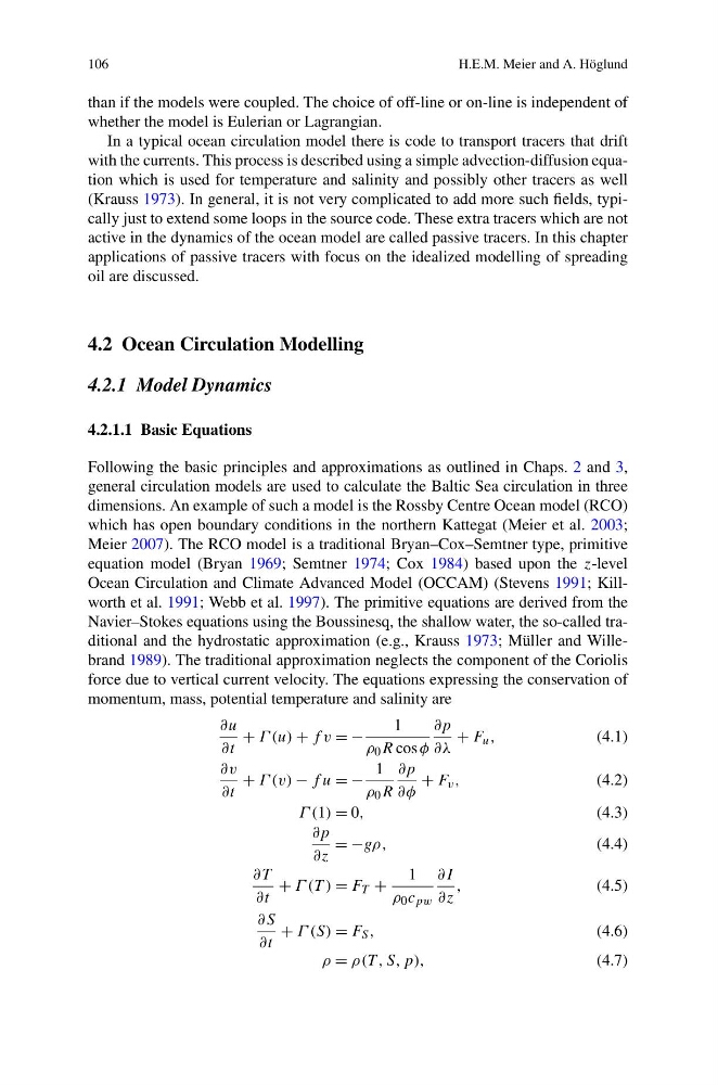
force due to vertical current velocity. The equations expressing the conservation of
momentum, mass, potential temperature and salinity are
∂u
∂t
+ Γ (u) + f v = −
1
ρ 0 R cos φ
∂p
∂λ
+ F u ,
(4.1)
∂v
∂t
+ Γ (v) − f u = −
1
ρ 0 R
∂p
∂φ
+ F v ,
(4.2)
Γ (1) = 0,
(4.3)
∂p
∂z
= −gρ,
(4.4)
∂T
∂t
+ Γ (T ) = F T +
1
ρ 0 c pw
∂I
∂z
,
(4.5)
∂S
∂t
+ Γ (S) = F S ,
(4.6)
ρ = ρ(T , S, p),
(4.7)
H.E.M. Meier and A. Höglund
than if the models were coupled. The choice of off-line or on-line is independent of
whether the model is Eulerian or Lagrangian.
In a typical ocean circulation model there is code to transport tracers that drift
with the currents. This process is described using a simple advection-diffusion equation which is used for temperature and salinity and possibly other tracers as well
(Krauss 1973). In general, it is not very complicated to add more such fields, typically just to extend some loops in the source code. These extra tracers which are not
active in the dynamics of the ocean model are called passive tracers. In this chapter
applications of passive tracers with focus on the idealized modelling of spreading
oil are discussed.
4.2 Ocean Circulation Modelling
4.2.1 Model Dynamics
4.2.1.1 Basic Equations
Following the basic principles and approximations as outlined in Chaps. 2 and 3,
general circulation models are used to calculate the Baltic Sea circulation in three
dimensions. An example of such a model is the Rossby Centre Ocean model (RCO)
which has open boundary conditions in the northern Kattegat (Meier et al. 2003;
Meier 2007). The RCO model is a traditional Bryan–Cox–Semtner type, primitive
equation model (Bryan 1969; Semtner 1974; Cox 1984) based upon the z-level
Ocean Circulation and Climate Advanced Model (OCCAM) (Stevens 1991; Killworth et al. 1991; Webb et al. 1997). The primitive equations are derived from the
Navier–Stokes equations using the Boussinesq, the shallow water, the so-called traditional and the hydrostatic approximation (e.g., Krauss 1973; Müller and Willebrand 1989). The traditional approximation neglects the component of the Coriolis
force due to vertical current velocity. The equations expressing the conservation of
momentum, mass, potential temperature and salinity are
∂u
∂t
+ Γ (u) + f v = −
1
ρ 0 R cos φ
∂p
∂λ
+ F u ,
(4.1)
∂v
∂t
+ Γ (v) − f u = −
1
ρ 0 R
∂p
∂φ
+ F v ,
(4.2)
Γ (1) = 0,
(4.3)
∂p
∂z
= −gρ,
(4.4)
∂T
∂t
+ Γ (T ) = F T +
1
ρ 0 c pw
∂I
∂z
,
(4.5)
∂S
∂t
+ Γ (S) = F S ,
(4.6)
ρ = ρ(T , S, p),
(4.7)