38.1 Introduction
The transportation problem, in its classical formulation involves sources
(S i ) i 2 {1, . . . , n} , where supplies (s i ) i ¼ 1 , . . . , n of some goods are available, and
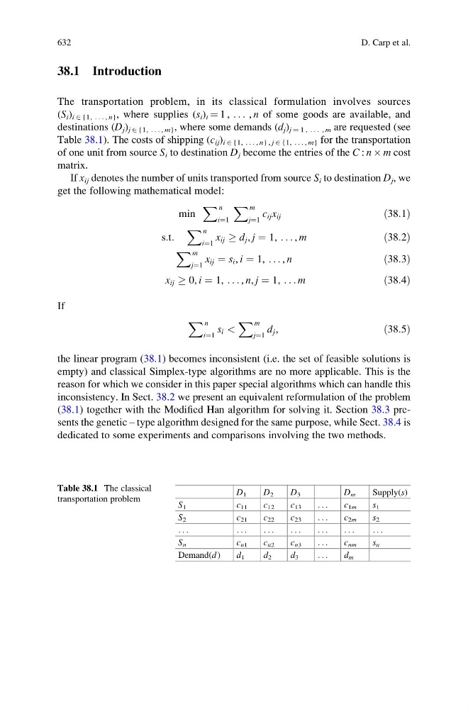
destinations (D j ) j 2 {1, . . . , m} , where some demands (d j ) j ¼ 1 , . . . , m are requested (see
Table 38.1). The costs of shipping (c ij ) i 2 {1, . . . , n} , j 2 {1, . . . , m} for the transportation
of one unit from source S i to destination D j become the entries of the C : n  m cost
matrix.
If x ij denotes the number of units transported from source S i to destination D j , we
get the following mathematical model:
min
X n
i¼1
X m
j¼1
c ij x ij
ð38:1Þ
s:t:
X n
i¼1
x ij ! d j , j ¼ 1, . . . , m
ð38:2Þ
X m
j¼1
x ij ¼ s i , i ¼ 1, . . . , n
ð38:3Þ
x ij ! 0, i ¼ 1, . . . , n, j ¼ 1, . . . m
ð38:4Þ
If
X n
i¼1
s i <
X m
j¼1
d j ,
ð38:5Þ
the linear program (38.1) becomes inconsistent (i.e. the set of feasible solutions is
empty) and classical Simplex-type algorithms are no more applicable. This is the
reason for which we consider in this paper special algorithms which can handle this
inconsistency. In Sect. 38.2 we present an equivalent reformulation of the problem
(38.1) together with the Modified Han algorithm for solving it. Section 38.3 presents the genetic – type algorithm designed for the same purpose, while Sect. 38.4 is
dedicated to some experiments and comparisons involving the two methods.
Table 38.1 The classical
transportation problem
D 1
D 2
D 3
D m
Supply(s)
S 1
c 11
c 12
c 13
. . .
c 1m
s 1
S 2
c 21
c 22
c 23
. . .
c 2m
s 2
. . .
. . .
. . .
. . .
. . .
. . .
. . .
S n
c n1
c n2
c n3
. . .
c nm
s n
Demand(d )
d 1
d 2
d 3
. . .
d m
632
D. Carp et al.