

OPTION 2
Predator-Prey Interactions
243
be attempted simultaneously. Each laboratory team should be responsible for one
or two prey densities, with each predator tested separately. While feeding is in
progress, carefully observe the behavior of each predator. Allow 3 min for feeding,
remove the predators, and count the number of prey remaining. At high prey
densities, record predator strikes and successful captures; confusion of the predator
can occur at high prey densities with an increase in strikes but a decline in capture,
particularly by the fish. Record the number of prey consumed by each predator
at each prey density.
4. Graph the relationship between prey density and prey consumed for each predator
type. Include the results of the trials done in the light (15 prey per container), above,
with the data from this part.
5. Optional experimental variations:
a. Feed predators live and dead prey and observe the differences.
b. Compare fish attacks on clear test tubes containing different sizes of Daphnia
prey.
c. Place small red and blue dots on a flask or the aquaria and observe the fish
feeding behavior.
d. Try repeating fish predation experiments with different backgrounds (paper or
boxes) around beakers, or while shining differently colored lights on the beakers.
e. Place the Daphnia in one of several suspensions of food color for ca. 15 min
and repeat fish predation experiments. What effect does color have?
Questions
1. Evaluate the plots of feeding data for each predator.
a. What does the shape of each curve suggest about the predator?
b. How do the curves compare?
c. What factors appear to be responsible for the observed responses?
d. How reliable are these data for extrapolation to natural environments?
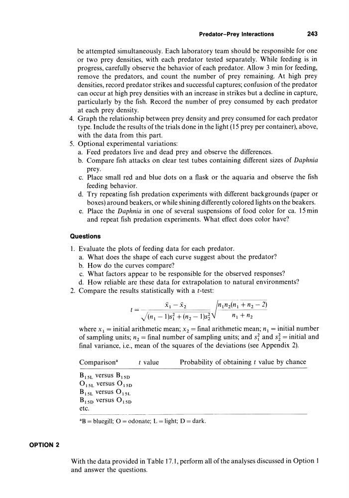
2. Compare the results statistically with at-test:
Xl - Xl
Jn 1nz(n 1 + nl - 2)
t-~====~======~
J(n 1 - l)si + (nl - l)s~
n1 + n2
where Xl = initial arithmetic mean; X 2 = final arithmetic mean; n 1 = initial number
of sampling units; n 2 = final number of sampling units; and si and s~ = initial and
final variance, i.e., mean of the squares of the deviations (see Appendix 2).
Comparison a
B 15L versus B 150
015L versus 0 150
B15L versus 015L
B 150 versus 0 150
etc.
t value
Probability of obtaining t value by chance
aB = bluegill; 0 = odonate; L = light; D = dark.
With the data provided in Table 17.1, perform all of the analyses discussed in Option 1
and answer the questions.
Predator-Prey Interactions
243
be attempted simultaneously. Each laboratory team should be responsible for one
or two prey densities, with each predator tested separately. While feeding is in
progress, carefully observe the behavior of each predator. Allow 3 min for feeding,
remove the predators, and count the number of prey remaining. At high prey
densities, record predator strikes and successful captures; confusion of the predator
can occur at high prey densities with an increase in strikes but a decline in capture,
particularly by the fish. Record the number of prey consumed by each predator
at each prey density.
4. Graph the relationship between prey density and prey consumed for each predator
type. Include the results of the trials done in the light (15 prey per container), above,
with the data from this part.
5. Optional experimental variations:
a. Feed predators live and dead prey and observe the differences.
b. Compare fish attacks on clear test tubes containing different sizes of Daphnia
prey.
c. Place small red and blue dots on a flask or the aquaria and observe the fish
feeding behavior.
d. Try repeating fish predation experiments with different backgrounds (paper or
boxes) around beakers, or while shining differently colored lights on the beakers.
e. Place the Daphnia in one of several suspensions of food color for ca. 15 min
and repeat fish predation experiments. What effect does color have?
Questions
1. Evaluate the plots of feeding data for each predator.
a. What does the shape of each curve suggest about the predator?
b. How do the curves compare?
c. What factors appear to be responsible for the observed responses?
d. How reliable are these data for extrapolation to natural environments?
2. Compare the results statistically with at-test:
Xl - Xl
Jn 1nz(n 1 + nl - 2)
t-~====~======~
J(n 1 - l)si + (nl - l)s~
n1 + n2
where Xl = initial arithmetic mean; X 2 = final arithmetic mean; n 1 = initial number
of sampling units; n 2 = final number of sampling units; and si and s~ = initial and
final variance, i.e., mean of the squares of the deviations (see Appendix 2).
Comparison a
B 15L versus B 150
015L versus 0 150
B15L versus 015L
B 150 versus 0 150
etc.
t value
Probability of obtaining t value by chance
aB = bluegill; 0 = odonate; L = light; D = dark.
With the data provided in Table 17.1, perform all of the analyses discussed in Option 1
and answer the questions.