

Chapter 1: INTRODUCTION
1.7.1 Ekman boundary layer
The theory of the planetary boundary layer formulated by Ekman (1905)
provides a convenient framework for the analysis of the Earth’s rotation
effects. Here we present this theory in a manner close to that of Stull (1988)
and Mellor (1996).
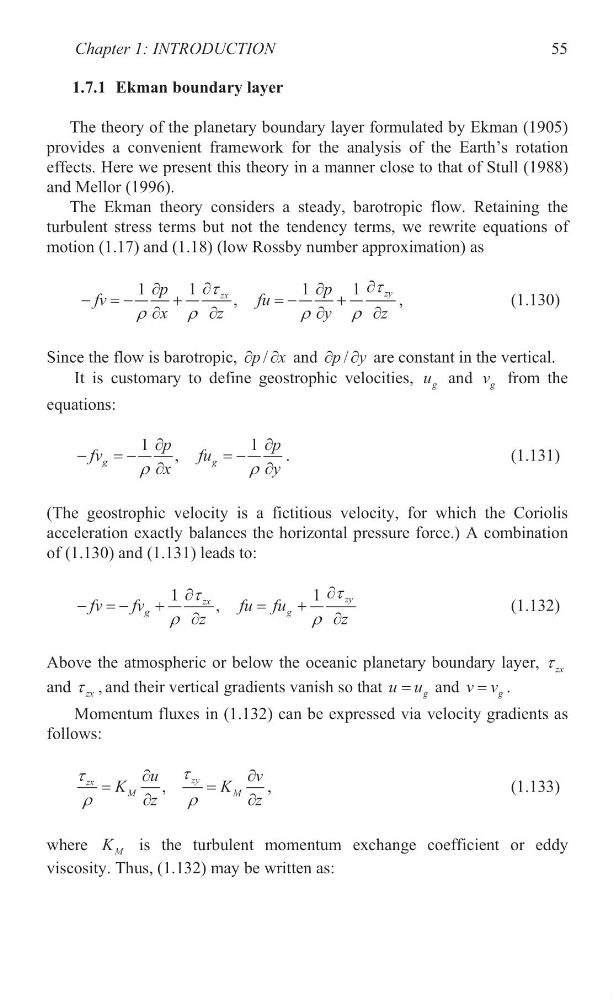
The Ekman theory considers a steady, barotropic flow. Retaining the
turbulent stress terms but not the tendency terms, we rewrite equations of
motion (1.17) and (1.18) (low Rossby number approximation) as
1
1
1
1
,
zy
zx
p
p
fv
fu
x
z
y
z
W
W
U
U
U
U
w
w
w
w
w
w
w
w
,
(1.130)
Since the flow is barotropic,
/
p x
w w and
/
p y
w w are constant in the vertical.
It is customary to define geostrophic velocities, g
u and g
v from the
equations:
1
1
,
g
g
p
p
fv
fu
x
y
U
U
w
w
w
w
.
(1.131)
(The geostrophic velocity is a fictitious velocity, for which the Coriolis
acceleration exactly balances the horizontal pressure force.) A combination
of (1.130) and (1.131) leads to:
1
1
,
zy
zx
g
g
fv
fv
fu fu
z
z
W
W
U
U
w
w
w
w
(1.132)
Above the atmospheric or below the oceanic planetary boundary layer, zx
W
and zx
W , and their vertical gradients vanish so that
g
u u and
g
v v .
Momentum fluxes in (1.132) can be expressed via velocity gradients as
follows:
,
zy
zx
M
M
u
v
K
K
z
z
W
W
U
U
w
w
w
w
,
(1.133)
where
M
K
is the turbulent momentum exchange coefficient or eddy
viscosity. Thus, (1.132) may be written as:
55
1.7.1 Ekman boundary layer
The theory of the planetary boundary layer formulated by Ekman (1905)
provides a convenient framework for the analysis of the Earth’s rotation
effects. Here we present this theory in a manner close to that of Stull (1988)
and Mellor (1996).
The Ekman theory considers a steady, barotropic flow. Retaining the
turbulent stress terms but not the tendency terms, we rewrite equations of
motion (1.17) and (1.18) (low Rossby number approximation) as
1
1
1
1
,
zy
zx
p
p
fv
fu
x
z
y
z
W
W
U
U
U
U
w
w
w
w
w
w
w
w
,
(1.130)
Since the flow is barotropic,
/
p x
w w and
/
p y
w w are constant in the vertical.
It is customary to define geostrophic velocities, g
u and g
v from the
equations:
1
1
,
g
g
p
p
fv
fu
x
y
U
U
w
w
w
w
.
(1.131)
(The geostrophic velocity is a fictitious velocity, for which the Coriolis
acceleration exactly balances the horizontal pressure force.) A combination
of (1.130) and (1.131) leads to:
1
1
,
zy
zx
g
g
fv
fv
fu fu
z
z
W
W
U
U
w
w
w
w
(1.132)
Above the atmospheric or below the oceanic planetary boundary layer, zx
W
and zx
W , and their vertical gradients vanish so that
g
u u and
g
v v .
Momentum fluxes in (1.132) can be expressed via velocity gradients as
follows:
,
zy
zx
M
M
u
v
K
K
z
z
W
W
U
U
w
w
w
w
,
(1.133)
where
M
K
is the turbulent momentum exchange coefficient or eddy
viscosity. Thus, (1.132) may be written as:
55