

For comparison, the spectrum of integrated acceleration is also shown in
Figure 3-7a. The acceleration spectrum suggests that the vibration
“contamination” occurs in narrow frequency bands. Further evidence of the
nature and degree of the vibration contamination can be seen in the plot of
Chapter 3: NEAR-SURFACE TURBULENCE
165
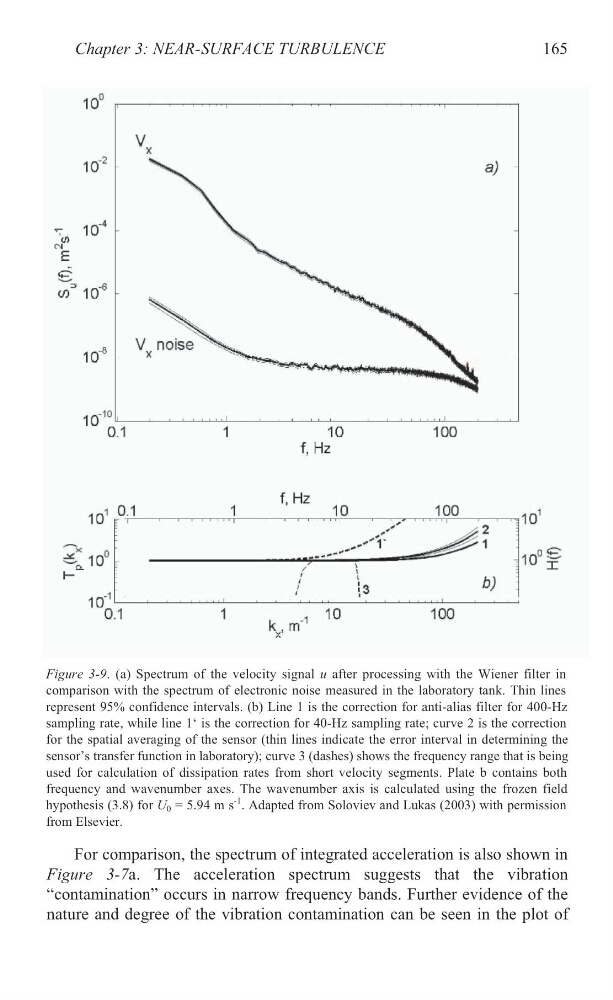
Figure 3-9. (a) Spectrum of the velocity signal u after processing with the Wiener filter in
comparison with the spectrum of electronic noise measured in the laboratory tank. Thin lines
represent 95% confidence intervals. (b) Line 1 is the correction for anti-alias filter for 400-Hz
sampling rate, while line 1‘ is the correction for 40-Hz sampling rate; curve 2 is the correction
for the spatial averaging of the sensor (thin lines indicate the error interval in determining the
sensor’s transfer function in laboratory); curve 3 (dashes) shows the frequency range that is being
used for calculation of dissipation rates from short velocity segments. Plate b contains both
frequency and wavenumber axes. The wavenumber axis is calculated using the frozen field
hypothesis (3.8) for U 0 = 5.94 m s
-1
from Elsevier.
. Adapted from Soloviev and Lukas (2003) with permission
Figure 3-7a. The acceleration spectrum suggests that the vibration
“contamination” occurs in narrow frequency bands. Further evidence of the
nature and degree of the vibration contamination can be seen in the plot of
Chapter 3: NEAR-SURFACE TURBULENCE
165
Figure 3-9. (a) Spectrum of the velocity signal u after processing with the Wiener filter in
comparison with the spectrum of electronic noise measured in the laboratory tank. Thin lines
represent 95% confidence intervals. (b) Line 1 is the correction for anti-alias filter for 400-Hz
sampling rate, while line 1‘ is the correction for 40-Hz sampling rate; curve 2 is the correction
for the spatial averaging of the sensor (thin lines indicate the error interval in determining the
sensor’s transfer function in laboratory); curve 3 (dashes) shows the frequency range that is being
used for calculation of dissipation rates from short velocity segments. Plate b contains both
frequency and wavenumber axes. The wavenumber axis is calculated using the frozen field
hypothesis (3.8) for U 0 = 5.94 m s
-1
from Elsevier.
. Adapted from Soloviev and Lukas (2003) with permission