

Arctic Ocean Circulation
365
(a)
(b)
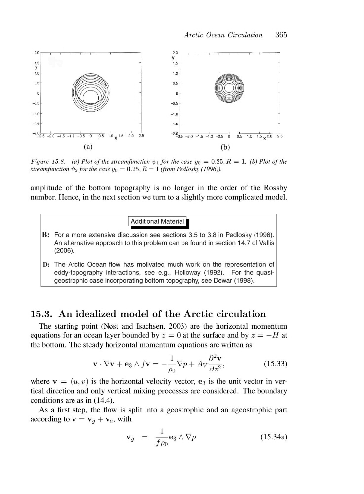
Figure 15.8. (a) Plot of the streamfunction ψ1 for the case y0 =0 .25,R =1 . (b) Plot of the
streamfunction ψ2 for the case y0 =0.25,R =1(from Pedlosky (1996)).
amplitude of the bottom topography is no longer in the order of the Rossby
number. Hence, in the next section we turn to a slightly more complicated model.
Additional Material
B: For a more extensive discussion see sections 3.5 to 3.8 in Pedlosky (1996).
An alternative approach to this problem can be found in section 14.7 of Vallis
(2006).
D: The Arctic Ocean flow has motivated much work on the representation of
eddy-topography interactions, see e.g., Holloway (1992). For the quasigeostrophic case incorporating bottom topography, see Dewar (1998).
15.3. An idealized model of the Arctic circulation
The starting point (Nøst and Isachsen, 2003) are the horizontal momentum
equations for an ocean layer bounded by z =0at the surface and by z = −H at
the bottom. The steady horizontal momentum equations are written as
v ·∇v + e 3 ∧ f v = −
1
ρ 0
∇p + A V
∂ 2 v
∂z 2 ,
(15.33)
where v =( u, v) is the horizontal velocity vector, e 3 is the unit vector in vertical direction and only vertical mixing processes are considered. The boundary
conditions are as in (14.4).
As a first step, the flow is split into a geostrophic and an ageostrophic part
according to v = v g + v a , with
v g =
1
fρ 0
e 3 ∧∇p
(15.34a)
365
(a)
(b)
Figure 15.8. (a) Plot of the streamfunction ψ1 for the case y0 =0 .25,R =1 . (b) Plot of the
streamfunction ψ2 for the case y0 =0.25,R =1(from Pedlosky (1996)).
amplitude of the bottom topography is no longer in the order of the Rossby
number. Hence, in the next section we turn to a slightly more complicated model.
Additional Material
B: For a more extensive discussion see sections 3.5 to 3.8 in Pedlosky (1996).
An alternative approach to this problem can be found in section 14.7 of Vallis
(2006).
D: The Arctic Ocean flow has motivated much work on the representation of
eddy-topography interactions, see e.g., Holloway (1992). For the quasigeostrophic case incorporating bottom topography, see Dewar (1998).
15.3. An idealized model of the Arctic circulation
The starting point (Nøst and Isachsen, 2003) are the horizontal momentum
equations for an ocean layer bounded by z =0at the surface and by z = −H at
the bottom. The steady horizontal momentum equations are written as
v ·∇v + e 3 ∧ f v = −
1
ρ 0
∇p + A V
∂ 2 v
∂z 2 ,
(15.33)
where v =( u, v) is the horizontal velocity vector, e 3 is the unit vector in vertical direction and only vertical mixing processes are considered. The boundary
conditions are as in (14.4).
As a first step, the flow is split into a geostrophic and an ageostrophic part
according to v = v g + v a , with
v g =
1
fρ 0
e 3 ∧∇p
(15.34a)