

362
DYNAMICAL OCEANOGRAPHY
◭
The example clearly shows that the upper-layer flow caused by the Ekman
pumping can deform the lower-layer geostrophic contours such that they can become closed. When closed, these contours are disconnected from the eastern
boundary and hence, in principle, flow is possible within such regions. But how
is it determined?
a
b
s
C
A
n
ds
σ`ds
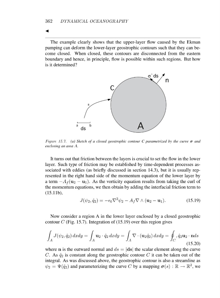
Figure 15.7. (a) Sketch of a closed geostrophic contour C parametrized by the curve σ and
enclosing an area A.
It turns out that friction between the layers is crucial to set the flow in the lower
layer. Such type of friction may be established by time-dependent processes associated with eddies (as briefly discussed in section 14.3), but it is usually represented in the right hand side of the momentum equation of the lower layer by
at e r m−A f (u 2 − u 1 ). As the vorticity equation results from taking the curl of
the momentum equations, we then obtain by adding the interfacial friction term to
(15.11b),
J(ψ 2 , ˆ
q 2 )=−ǫ 0 ∇
2 ψ 2 − A f ∇∧(u 2 − u 1 ).
(15.19)
Now consider a region A in the lower layer enclosed by a closed geostrophic
contour C (Fig. 15.7). Integration of (15.19) over this region gives
A
J(ψ 2 , ˆ
q 2 ) dxdy =
A
u 2 · ˆ
q 2 dxdy =
A
∇·(u 2 ˆ
q 2 ) dxdy =
C
, ˆ
q 2 u 2 · nds
(15.20)
where n is the outward normal and ds = |ds| the scalar element along the curve
C.A sˆ q 2 is constant along the geostrophic contour C it can be taken out of the
integral. As was discussed above, the geostrophic contour is also a streamline as
ψ 2 =Ψ (ˆ q 2 ) and parameterizing the curve C by a mapping σ(s):R → R 2 ,w e
DYNAMICAL OCEANOGRAPHY
◭
The example clearly shows that the upper-layer flow caused by the Ekman
pumping can deform the lower-layer geostrophic contours such that they can become closed. When closed, these contours are disconnected from the eastern
boundary and hence, in principle, flow is possible within such regions. But how
is it determined?
a
b
s
C
A
n
ds
σ`ds
Figure 15.7. (a) Sketch of a closed geostrophic contour C parametrized by the curve σ and
enclosing an area A.
It turns out that friction between the layers is crucial to set the flow in the lower
layer. Such type of friction may be established by time-dependent processes associated with eddies (as briefly discussed in section 14.3), but it is usually represented in the right hand side of the momentum equation of the lower layer by
at e r m−A f (u 2 − u 1 ). As the vorticity equation results from taking the curl of
the momentum equations, we then obtain by adding the interfacial friction term to
(15.11b),
J(ψ 2 , ˆ
q 2 )=−ǫ 0 ∇
2 ψ 2 − A f ∇∧(u 2 − u 1 ).
(15.19)
Now consider a region A in the lower layer enclosed by a closed geostrophic
contour C (Fig. 15.7). Integration of (15.19) over this region gives
A
J(ψ 2 , ˆ
q 2 ) dxdy =
A
u 2 · ˆ
q 2 dxdy =
A
∇·(u 2 ˆ
q 2 ) dxdy =
C
, ˆ
q 2 u 2 · nds
(15.20)
where n is the outward normal and ds = |ds| the scalar element along the curve
C.A sˆ q 2 is constant along the geostrophic contour C it can be taken out of the
integral. As was discussed above, the geostrophic contour is also a streamline as
ψ 2 =Ψ (ˆ q 2 ) and parameterizing the curve C by a mapping σ(s):R → R 2 ,w e