

332
DYNAMICAL OCEANOGRAPHY
Additional Material
B: A description of Antarctic Oceanography can be found in chapter 6 of Tomczak and Godfrey (1994). A more extensive discussion on the flow in the
Southern Ocean is given in section 4.6 of WOCE (2001).
14.2. The barotropic channel model
An idealized model of the ACC is that of a barotropic flow in a zonal channel
with a geometry as in Fig. 13.7. This channel is located in the Southern Hemisphere and it is bounded by latitudes θ = θ 1 and θ = θ 2 . The flow is forced at
the ocean-atmosphere interface by an idealized wind stress (τ φ ,τ θ ). The bottom
topography is represented by a function h b (φ, θ).
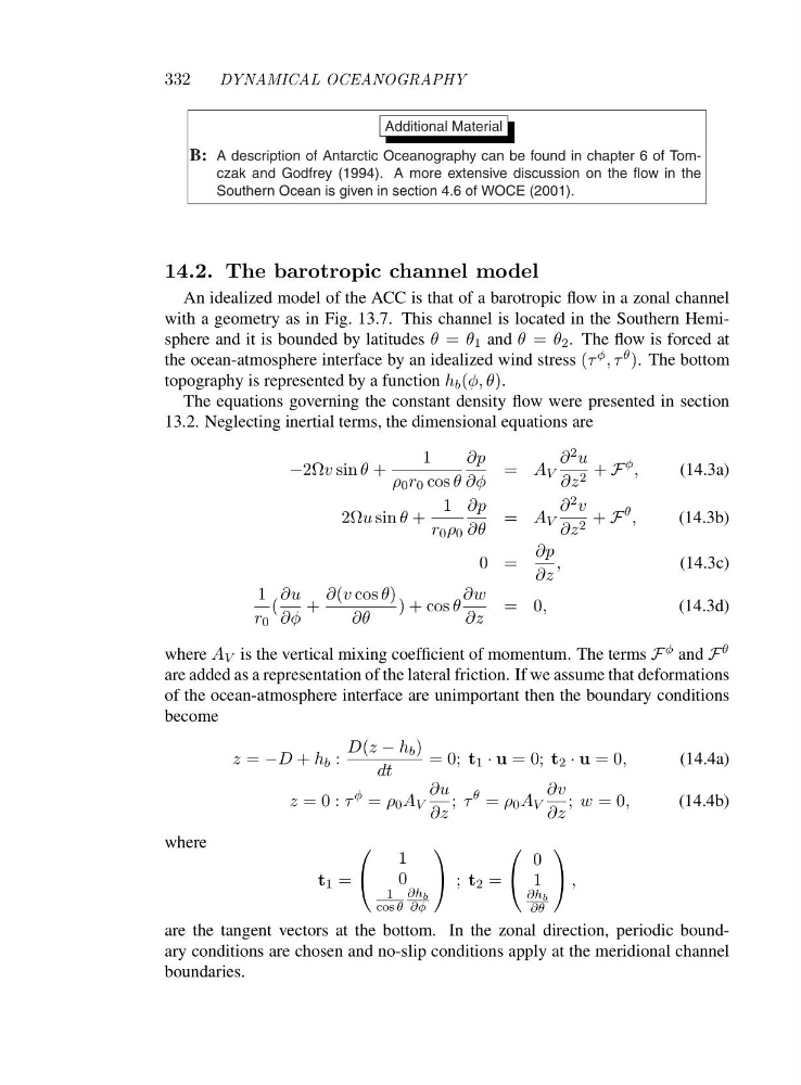
The equations governing the constant density flow were presented in section
13.2. Neglecting inertial terms, the dimensional equations are
−2Ωv sin θ +
1
ρ 0 r 0 cos θ
∂p
∂φ
= A V
∂ 2 u
∂z 2 + F
φ ,
(14.3a)
2Ωu sin θ +
1
r 0 ρ 0
∂p
∂θ
= A V
∂ 2 v
∂z 2 + F
θ ,
(14.3b)
0=
∂p
∂z
,
(14.3c)
1
r 0
(
∂u
∂φ
+
∂(v cos θ)
∂θ
)+cosθ
∂w
∂z
=0 ,
(14.3d)
where A V is the vertical mixing coefficient of momentum. The terms F φ and F θ
are added as a representation of the lateral friction. If we assume that deformations
of the ocean-atmosphere interface are unimportant then the boundary conditions
become
z = −D + h b :
D(z − h b )
dt
=0; t 1 · u =0; t 2 · u =0,
(14.4a)
z =0:τ
φ = ρ 0 A V
∂u
∂z
; τ
θ = ρ 0 A V
∂v
∂z
; w =0,
(14.4b)
where
t 1 =
⎛
⎝
1
0
1
cos θ
∂h b
∂φ
⎞
⎠ ; t 2 =
⎛
⎝
0
1
∂h b
∂θ
⎞
⎠ ,
are the tangent vectors at the bottom. In the zonal direction, periodic boundary conditions are chosen and no-slip conditions apply at the meridional channel
boundaries.
DYNAMICAL OCEANOGRAPHY
Additional Material
B: A description of Antarctic Oceanography can be found in chapter 6 of Tomczak and Godfrey (1994). A more extensive discussion on the flow in the
Southern Ocean is given in section 4.6 of WOCE (2001).
14.2. The barotropic channel model
An idealized model of the ACC is that of a barotropic flow in a zonal channel
with a geometry as in Fig. 13.7. This channel is located in the Southern Hemisphere and it is bounded by latitudes θ = θ 1 and θ = θ 2 . The flow is forced at
the ocean-atmosphere interface by an idealized wind stress (τ φ ,τ θ ). The bottom
topography is represented by a function h b (φ, θ).
The equations governing the constant density flow were presented in section
13.2. Neglecting inertial terms, the dimensional equations are
−2Ωv sin θ +
1
ρ 0 r 0 cos θ
∂p
∂φ
= A V
∂ 2 u
∂z 2 + F
φ ,
(14.3a)
2Ωu sin θ +
1
r 0 ρ 0
∂p
∂θ
= A V
∂ 2 v
∂z 2 + F
θ ,
(14.3b)
0=
∂p
∂z
,
(14.3c)
1
r 0
(
∂u
∂φ
+
∂(v cos θ)
∂θ
)+cosθ
∂w
∂z
=0 ,
(14.3d)
where A V is the vertical mixing coefficient of momentum. The terms F φ and F θ
are added as a representation of the lateral friction. If we assume that deformations
of the ocean-atmosphere interface are unimportant then the boundary conditions
become
z = −D + h b :
D(z − h b )
dt
=0; t 1 · u =0; t 2 · u =0,
(14.4a)
z =0:τ
φ = ρ 0 A V
∂u
∂z
; τ
θ = ρ 0 A V
∂v
∂z
; w =0,
(14.4b)
where
t 1 =
⎛
⎝
1
0
1
cos θ
∂h b
∂φ
⎞
⎠ ; t 2 =
⎛
⎝
0
1
∂h b
∂θ
⎞
⎠ ,
are the tangent vectors at the bottom. In the zonal direction, periodic boundary conditions are chosen and no-slip conditions apply at the meridional channel
boundaries.