

Thermocline problem
321
u sin θ = −
∂p
∂θ
,
(13.99b)
∂w
∂z
=0 ,
(13.99c)
ρ = −
∂p
∂z
,
(13.99d)
w
∂ρ
∂z
= λ
∂ 2 ρ
∂z 2 ,
(13.99e)
and it follows immediately that w = w(θ). The advection-diffusion balance for
the density can be integrated with the result
ρ(θ, z)=C 1 (θ)e
w(θ)z
λ V
+ C 2 (θ).
(13.100)
When w(θ) < 0 then C 1 =0, because otherwise the density becomes unbounded,
and hence ρ = ρ s (θ).W h e nw(θ) > 0 the solution becomes
ρ(θ, z)=(ρ s (θ) − ρ ∞ (θ))e
zw(θ)
λ V
+ ρ ∞ (θ),
(13.101)
where ρ ∞ (θ) is the density at z →∞ . Hence the characteristic vertical scale of
the density anomalies is λ/w(θ) and we can take h(θ)=λ V /w(θ) as a measure
of the depth of the thermocline. The corresponding dimensional vertical scale of
the thermocline is δ D .
◭
φ
θ
z
w E < 0
w E > 0
advective
diffusive
advective
w E = 0
δ D
δ a
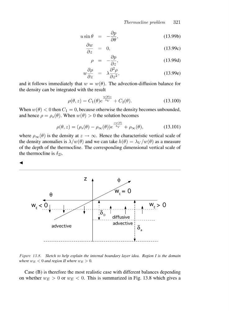
Figure 13.8. Sketch to help explain the internal boundary layer idea. Region I is the domain
where wE < 0 and region II where wE > 0.
Case (B) is therefore the most realistic case with different balances depending
on whether w E > 0 or w E < 0. This is summarized in Fig. 13.8 which gives a
321
u sin θ = −
∂p
∂θ
,
(13.99b)
∂w
∂z
=0 ,
(13.99c)
ρ = −
∂p
∂z
,
(13.99d)
w
∂ρ
∂z
= λ
∂ 2 ρ
∂z 2 ,
(13.99e)
and it follows immediately that w = w(θ). The advection-diffusion balance for
the density can be integrated with the result
ρ(θ, z)=C 1 (θ)e
w(θ)z
λ V
+ C 2 (θ).
(13.100)
When w(θ) < 0 then C 1 =0, because otherwise the density becomes unbounded,
and hence ρ = ρ s (θ).W h e nw(θ) > 0 the solution becomes
ρ(θ, z)=(ρ s (θ) − ρ ∞ (θ))e
zw(θ)
λ V
+ ρ ∞ (θ),
(13.101)
where ρ ∞ (θ) is the density at z →∞ . Hence the characteristic vertical scale of
the density anomalies is λ/w(θ) and we can take h(θ)=λ V /w(θ) as a measure
of the depth of the thermocline. The corresponding dimensional vertical scale of
the thermocline is δ D .
◭
φ
θ
z
w E < 0
w E > 0
advective
diffusive
advective
w E = 0
δ D
δ a
Figure 13.8. Sketch to help explain the internal boundary layer idea. Region I is the domain
where wE < 0 and region II where wE > 0.
Case (B) is therefore the most realistic case with different balances depending
on whether w E > 0 or w E < 0. This is summarized in Fig. 13.8 which gives a