

20
DYNAMICAL OCEANOGRAPHY
Characteristic
Notation
Value
Reference density
ρ 0
1.0 × 10 3 kgm −3
Heat Capacity
C p
4.2 × 10 3 Jkg −1 K −1
Thermal expansion coefficient
α T
1.0 × 10 −4 K −1
Haline expansion coefficient
α S
7.6 × 10 −4 −
Kinematic viscosity
ν
1.0 × 10 −6 m 2 s −1 .
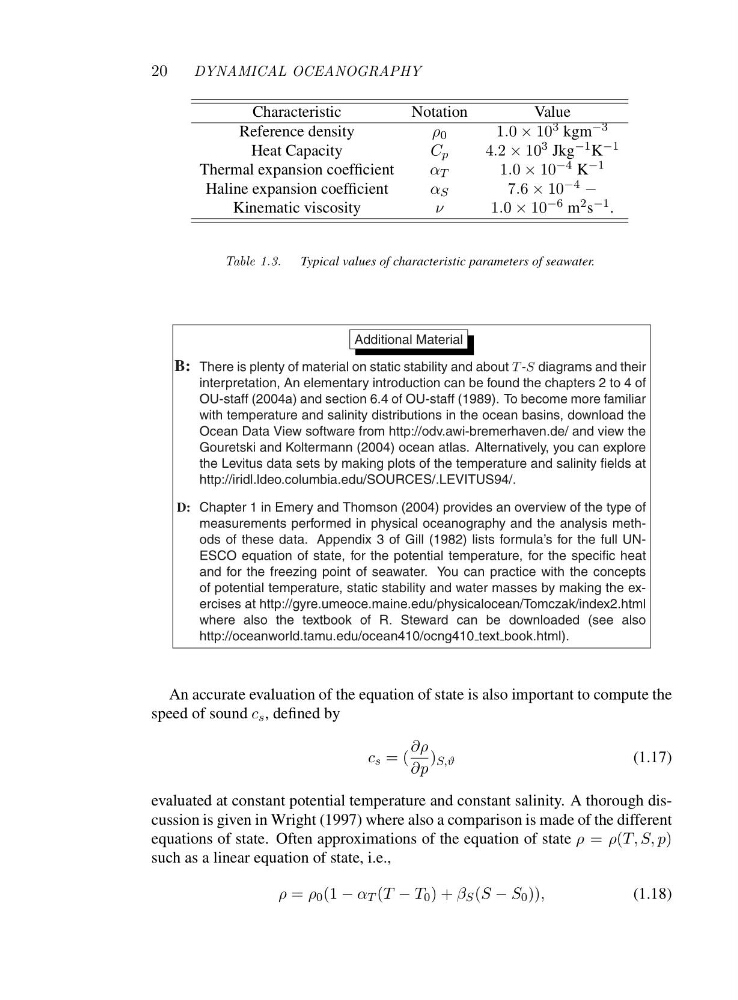
Table 1.3. Typical values of characteristic parameters of seawater.
Additional Material
B: There is plenty of material on static stability and about T -S diagrams and their
interpretation, An elementary introduction can be found the chapters 2 to 4 of
OU-staff (2004a) and section 6.4 of OU-staff (1989). To become more familiar
with temperature and salinity distributions in the ocean basins, download the
Ocean Data View software from http://odv.awi-bremerhaven.de/ and view the
Gouretski and Koltermann (2004) ocean atlas. Alternatively, you can explore
the Levitus data sets by making plots of the temperature and salinity fields at
http://iridl.ldeo.columbia.edu/SOURCES/.LEVITUS94/.
D: Chapter 1 in Emery and Thomson (2004) provides an overview of the type of
measurements performed in physical oceanography and the analysis methods of these data. Appendix 3 of Gill (1982) lists formula’s for the full UNESCO equation of state, for the potential temperature, for the specific heat
and for the freezing point of seawater. You can practice with the concepts
of potential temperature, static stability and water masses by making the exercises at http://gyre.umeoce.maine.edu/physicalocean/Tomczak/index2.html
where also the textbook of R. Steward can be downloaded (see also
http://oceanworld.tamu.edu/ocean410/ocng410 text book.html).
An accurate evaluation of the equation of state is also important to compute the
speed of sound c s ,definedby
c s =(
∂ρ
∂p
) S,ϑ
(1.17)
evaluated at constant potential temperature and constant salinity. A thorough discussion is given in Wright (1997) where also a comparison is made of the different
equations of state. Often approximations of the equation of state ρ = ρ(T,S,p)
such as a linear equation of state, i.e.,
ρ = ρ 0 (1 − α T (T − T 0 )+β S (S − S 0 )),
(1.18)
DYNAMICAL OCEANOGRAPHY
Characteristic
Notation
Value
Reference density
ρ 0
1.0 × 10 3 kgm −3
Heat Capacity
C p
4.2 × 10 3 Jkg −1 K −1
Thermal expansion coefficient
α T
1.0 × 10 −4 K −1
Haline expansion coefficient
α S
7.6 × 10 −4 −
Kinematic viscosity
ν
1.0 × 10 −6 m 2 s −1 .
Table 1.3. Typical values of characteristic parameters of seawater.
Additional Material
B: There is plenty of material on static stability and about T -S diagrams and their
interpretation, An elementary introduction can be found the chapters 2 to 4 of
OU-staff (2004a) and section 6.4 of OU-staff (1989). To become more familiar
with temperature and salinity distributions in the ocean basins, download the
Ocean Data View software from http://odv.awi-bremerhaven.de/ and view the
Gouretski and Koltermann (2004) ocean atlas. Alternatively, you can explore
the Levitus data sets by making plots of the temperature and salinity fields at
http://iridl.ldeo.columbia.edu/SOURCES/.LEVITUS94/.
D: Chapter 1 in Emery and Thomson (2004) provides an overview of the type of
measurements performed in physical oceanography and the analysis methods of these data. Appendix 3 of Gill (1982) lists formula’s for the full UNESCO equation of state, for the potential temperature, for the specific heat
and for the freezing point of seawater. You can practice with the concepts
of potential temperature, static stability and water masses by making the exercises at http://gyre.umeoce.maine.edu/physicalocean/Tomczak/index2.html
where also the textbook of R. Steward can be downloaded (see also
http://oceanworld.tamu.edu/ocean410/ocng410 text book.html).
An accurate evaluation of the equation of state is also important to compute the
speed of sound c s ,definedby
c s =(
∂ρ
∂p
) S,ϑ
(1.17)
evaluated at constant potential temperature and constant salinity. A thorough discussion is given in Wright (1997) where also a comparison is made of the different
equations of state. Often approximations of the equation of state ρ = ρ(T,S,p)
such as a linear equation of state, i.e.,
ρ = ρ 0 (1 − α T (T − T 0 )+β S (S − S 0 )),
(1.18)