

280
DYNAMICAL OCEANOGRAPHY
H
m
Q oa
Q
b
w
*
T r*
T
*
T
s*
-
z = 0
z
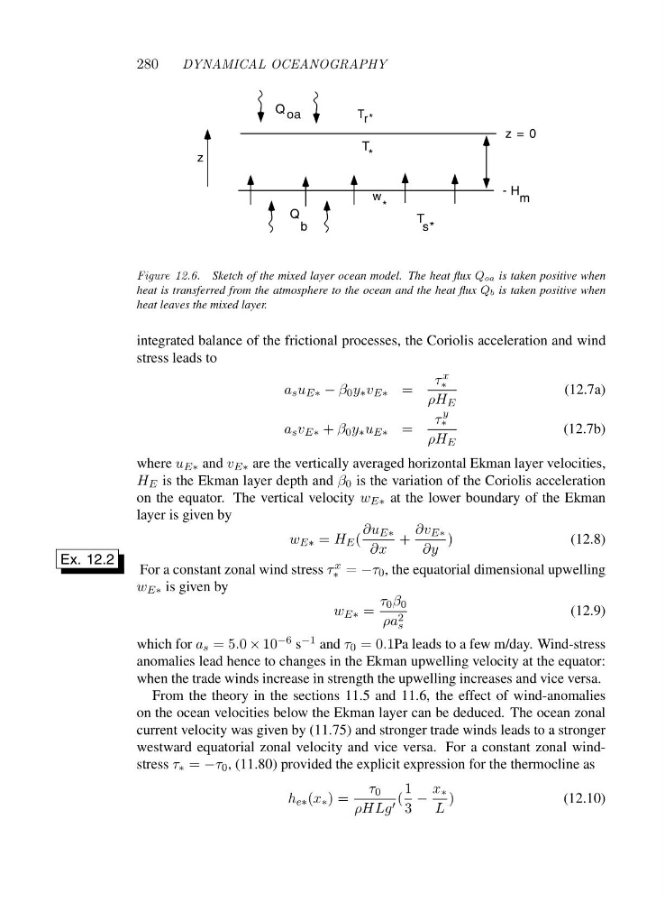
Figure 12.6. Sketch of the mixed layer ocean model. The heat flux Qoa is taken positive when
heat is transferred from the atmosphere to the ocean and the heat flux Qb is taken positive when
heat leaves the mixed layer.
integrated balance of the frictional processes, the Coriolis acceleration and wind
stress leads to
a s u E∗ − β 0 y ∗ v E∗ =
τ x
∗
ρH E
(12.7a)
a s v E∗ + β 0 y ∗ u E∗ =
τ
y
∗
ρH E
(12.7b)
where u E∗ and v E∗ are the vertically averaged horizontal Ekman layer velocities,
H E is the Ekman layer depth and β 0 is the variation of the Coriolis acceleration
on the equator. The vertical velocity w E∗ at the lower boundary of the Ekman
layer is given by
w E∗ = H E (
∂u E∗
∂x
+
∂v E∗
∂y
)
(12.8)
For a constant zonal wind stress τ x
∗ = −τ 0 , the equatorial dimensional upwelling
Ex. 12.2
w E∗ is given by
w E∗ =
τ 0 β 0
ρa 2
s
(12.9)
which for a s =5.0 × 10 −6 s −1 and τ 0 =0.1Pa leads to a few m/day. Wind-stress
anomalies lead hence to changes in the Ekman upwelling velocity at the equator:
when the trade winds increase in strength the upwelling increases and vice versa.
From the theory in the sections 11.5 and 11.6, the effect of wind-anomalies
on the ocean velocities below the Ekman layer can be deduced. The ocean zonal
current velocity was given by (11.75) and stronger trade winds leads to a stronger
westward equatorial zonal velocity and vice versa. For a constant zonal windstress τ ∗ = −τ 0 , (11.80) provided the explicit expression for the thermocline as
h e∗ (x ∗ )=
τ 0
ρHLg ′ (
1
3
−
x ∗
L
)
(12.10)
DYNAMICAL OCEANOGRAPHY
H
m
Q oa
Q
b
w
*
T r*
T
*
T
s*
-
z = 0
z
Figure 12.6. Sketch of the mixed layer ocean model. The heat flux Qoa is taken positive when
heat is transferred from the atmosphere to the ocean and the heat flux Qb is taken positive when
heat leaves the mixed layer.
integrated balance of the frictional processes, the Coriolis acceleration and wind
stress leads to
a s u E∗ − β 0 y ∗ v E∗ =
τ x
∗
ρH E
(12.7a)
a s v E∗ + β 0 y ∗ u E∗ =
τ
y
∗
ρH E
(12.7b)
where u E∗ and v E∗ are the vertically averaged horizontal Ekman layer velocities,
H E is the Ekman layer depth and β 0 is the variation of the Coriolis acceleration
on the equator. The vertical velocity w E∗ at the lower boundary of the Ekman
layer is given by
w E∗ = H E (
∂u E∗
∂x
+
∂v E∗
∂y
)
(12.8)
For a constant zonal wind stress τ x
∗ = −τ 0 , the equatorial dimensional upwelling
Ex. 12.2
w E∗ is given by
w E∗ =
τ 0 β 0
ρa 2
s
(12.9)
which for a s =5.0 × 10 −6 s −1 and τ 0 =0.1Pa leads to a few m/day. Wind-stress
anomalies lead hence to changes in the Ekman upwelling velocity at the equator:
when the trade winds increase in strength the upwelling increases and vice versa.
From the theory in the sections 11.5 and 11.6, the effect of wind-anomalies
on the ocean velocities below the Ekman layer can be deduced. The ocean zonal
current velocity was given by (11.75) and stronger trade winds leads to a stronger
westward equatorial zonal velocity and vice versa. For a constant zonal windstress τ ∗ = −τ 0 , (11.80) provided the explicit expression for the thermocline as
h e∗ (x ∗ )=
τ 0
ρHLg ′ (
1
3
−
x ∗
L
)
(12.10)