

Equatorial ocean circulation
255
(a)
(b)
(c)
(d)
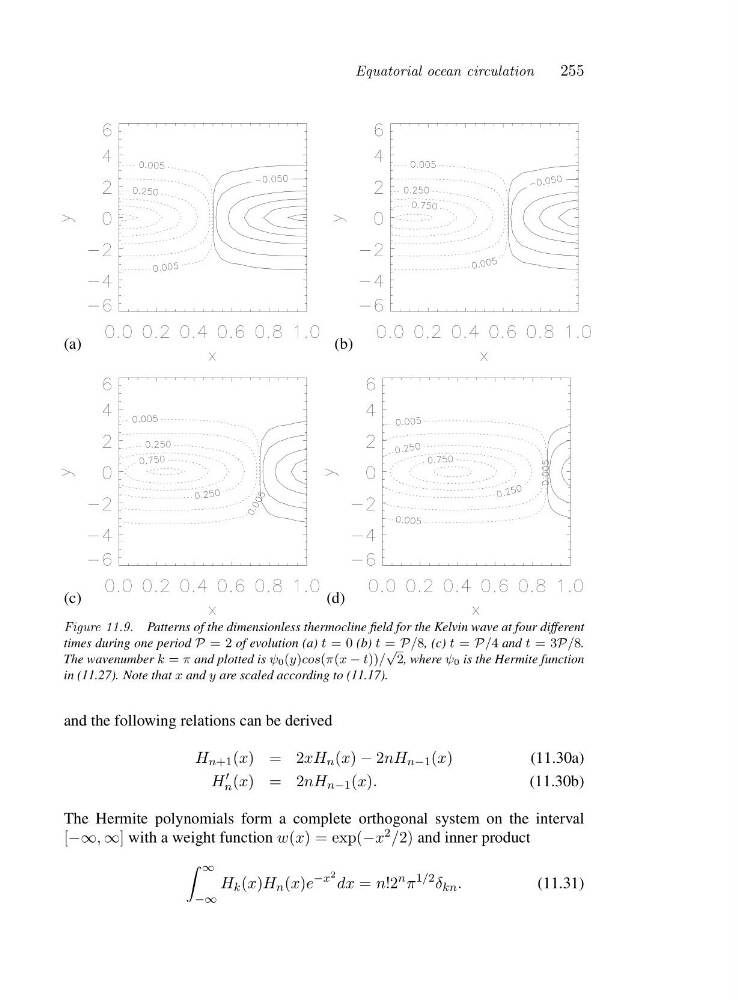
Figure 11.9. Patterns of the dimensionless thermocline field for the Kelvin wave at four different
times during one period P =2of evolution (a) t =0(b) t = P/8,(c)t = P/4 and t =3 P/8.
The wavenumber k = π and plotted is ψ0(y)cos(π(x − t))/
√
2,whereψ0 is the Hermite function
in (11.27). Note that x and y are scaled according to (11.17).
and the following relations can be derived
H n+1 (x)=2 xH n (x) − 2nH n−1 (x)
(11.30a)
H
′
n (x)=2 nH n−1 (x).
(11.30b)
The Hermite polynomials form a complete orthogonal system on the interval
[−∞, ∞] with a weight function w(x) = exp(−x 2 /2) and inner product
∞
−∞
H k (x)H n (x)e
−x 2 dx = n!2
n π
1/2 δ kn .
(11.31)
255
(a)
(b)
(c)
(d)
Figure 11.9. Patterns of the dimensionless thermocline field for the Kelvin wave at four different
times during one period P =2of evolution (a) t =0(b) t = P/8,(c)t = P/4 and t =3 P/8.
The wavenumber k = π and plotted is ψ0(y)cos(π(x − t))/
√
2,whereψ0 is the Hermite function
in (11.27). Note that x and y are scaled according to (11.17).
and the following relations can be derived
H n+1 (x)=2 xH n (x) − 2nH n−1 (x)
(11.30a)
H
′
n (x)=2 nH n−1 (x).
(11.30b)
The Hermite polynomials form a complete orthogonal system on the interval
[−∞, ∞] with a weight function w(x) = exp(−x 2 /2) and inner product
∞
−∞
H k (x)H n (x)e
−x 2 dx = n!2
n π
1/2 δ kn .
(11.31)