

Equatorial ocean circulation
253
∂v ∗
∂t ∗
+ β 0 y ∗ u ∗ = −g
′ ∂h ∗
∂y ∗
,
(11.16b)
∂h ∗
∂t ∗
+ H(
∂u ∗
∂x ∗
+
∂v ∗
∂y ∗
)=0 .
(11.16c)
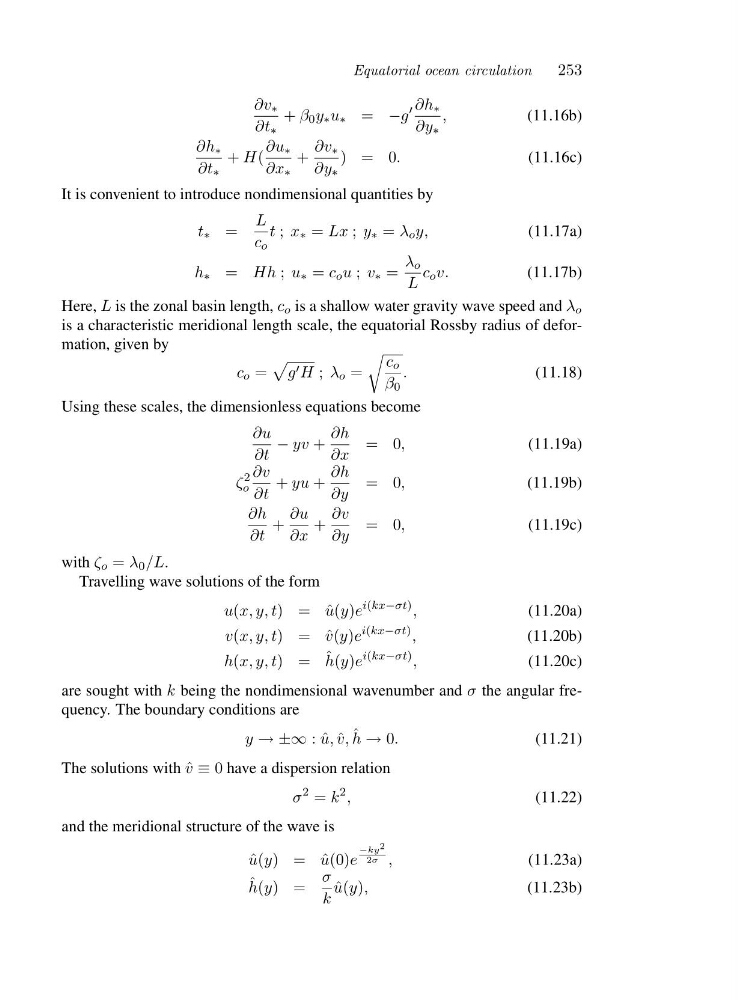
It is convenient to introduce nondimensional quantities by
t ∗ =
L
c o
t ; x ∗ = Lx ; y ∗ = λ o y,
(11.17a)
h ∗ = Hh ; u ∗ = c o u ; v ∗ =
λ o
L
c o v.
(11.17b)
Here, L is the zonal basin length, c o is a shallow water gravity wave speed and λ o
is a characteristic meridional length scale, the equatorial Rossby radius of deformation, given by
c o =
g ′ H ; λ o =
c o
β 0
.
(11.18)
Using these scales, the dimensionless equations become
∂u
∂t
− yv +
∂h
∂x
=0 ,
(11.19a)
ζ
2
o
∂v
∂t
+ yu +
∂h
∂y
=0 ,
(11.19b)
∂h
∂t
+
∂u
∂x
+
∂v
∂y
=0 ,
(11.19c)
with ζ o = λ 0 /L.
Travelling wave solutions of the form
u(x, y, t)=ˆ u(y)e
i(kx−σt) ,
(11.20a)
v(x, y, t)=ˆ v(y)e
i(kx−σt) ,
(11.20b)
h(x, y, t)= ˆ
h(y)e
i(kx−σt) ,
(11.20c)
are sought with k being the nondimensional wavenumber and σ the angular frequency. The boundary conditions are
y →±∞:ˆ u, ˆ
v, ˆ
h → 0.
(11.21)
The solutions with ˆ
v ≡ 0 have a dispersion relation
σ
2 = k
2 ,
(11.22)
and the meridional structure of the wave is
ˆ
u(y)=ˆ u(0)e
−ky 2
2σ ,
(11.23a)
ˆ
h(y)=
σ
k
ˆ
u(y),
(11.23b)
253
∂v ∗
∂t ∗
+ β 0 y ∗ u ∗ = −g
′ ∂h ∗
∂y ∗
,
(11.16b)
∂h ∗
∂t ∗
+ H(
∂u ∗
∂x ∗
+
∂v ∗
∂y ∗
)=0 .
(11.16c)
It is convenient to introduce nondimensional quantities by
t ∗ =
L
c o
t ; x ∗ = Lx ; y ∗ = λ o y,
(11.17a)
h ∗ = Hh ; u ∗ = c o u ; v ∗ =
λ o
L
c o v.
(11.17b)
Here, L is the zonal basin length, c o is a shallow water gravity wave speed and λ o
is a characteristic meridional length scale, the equatorial Rossby radius of deformation, given by
c o =
g ′ H ; λ o =
c o
β 0
.
(11.18)
Using these scales, the dimensionless equations become
∂u
∂t
− yv +
∂h
∂x
=0 ,
(11.19a)
ζ
2
o
∂v
∂t
+ yu +
∂h
∂y
=0 ,
(11.19b)
∂h
∂t
+
∂u
∂x
+
∂v
∂y
=0 ,
(11.19c)
with ζ o = λ 0 /L.
Travelling wave solutions of the form
u(x, y, t)=ˆ u(y)e
i(kx−σt) ,
(11.20a)
v(x, y, t)=ˆ v(y)e
i(kx−σt) ,
(11.20b)
h(x, y, t)= ˆ
h(y)e
i(kx−σt) ,
(11.20c)
are sought with k being the nondimensional wavenumber and σ the angular frequency. The boundary conditions are
y →±∞:ˆ u, ˆ
v, ˆ
h → 0.
(11.21)
The solutions with ˆ
v ≡ 0 have a dispersion relation
σ
2 = k
2 ,
(11.22)
and the meridional structure of the wave is
ˆ
u(y)=ˆ u(0)e
−ky 2
2σ ,
(11.23a)
ˆ
h(y)=
σ
k
ˆ
u(y),
(11.23b)