

232
DYNAMICAL OCEANOGRAPHY
The eigenfunctions are
Φ n (y)=A n cos l j y, l j =(j +
1
2
)π,
(10.54)
and substitution of these solutions into (10.52) leads to a set of homogeneous
equations for the A n . Setting the coefficient determinant to zero provides the
eigenvalues c as
c = U 2 +
U s K 2 (K 2 +2F 2 ) − β(2K 2 + F 1 + F 2 )
2K 2 (K 2 + F 1 + F 2 )
±
[β 2 (F 1 + F 2 ) 2 +2βU s K 4 (F 1 − F 2 ) − K 4 U 2
s (4F 1 F 2 − K 4 )]
1
2
K 2 (K 2 + F 1 + F 2 )
, (10.55)
with K 2 = k 2 + l 2
j . In the case U 1 = U 2 = U , we find two real eigenvalues
c 1 = U −
β
K 2 ,
(10.56a)
c 2 = U −
β
K 2 + F 1 + F 2
,
(10.56b)
and, apart from an additive constant, we find the phase speeds of the Rossby waves
of the first baroclinic mode (c 2 ) and the barotropic mode (c 1 ) (cf. section 9.2).
0
1
2
3
4
5
0
0.5
1
1.5
2
K
2
/F
FU
sc
/β β
β
β
unstable
stable
c
i
= 0
(a)
0
0.2
0.4
0.6
0.8
1
0
0.5
1
1.5
2
K
2
/F
c
i
/β β β
β
U
s
= 2 * U
sc
(b)
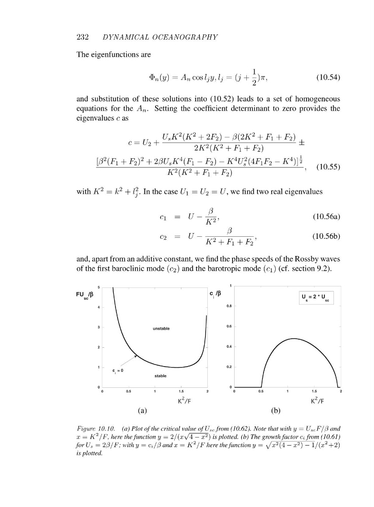
Figure 10.10. (a) Plot of the critical value of Usc from (10.62). Note that with y = UscF/β and
x = K
2 /F , here the function y =2/(x
√
4 − x 2 ) is plotted. (b) The growth factor ci from (10.61)
for Us =2β/F; with y = ci/β and x = K
2 /F here the function y =
x 2 (4 − x 2 ) − 1/(x
2 +2)
is plotted.
DYNAMICAL OCEANOGRAPHY
The eigenfunctions are
Φ n (y)=A n cos l j y, l j =(j +
1
2
)π,
(10.54)
and substitution of these solutions into (10.52) leads to a set of homogeneous
equations for the A n . Setting the coefficient determinant to zero provides the
eigenvalues c as
c = U 2 +
U s K 2 (K 2 +2F 2 ) − β(2K 2 + F 1 + F 2 )
2K 2 (K 2 + F 1 + F 2 )
±
[β 2 (F 1 + F 2 ) 2 +2βU s K 4 (F 1 − F 2 ) − K 4 U 2
s (4F 1 F 2 − K 4 )]
1
2
K 2 (K 2 + F 1 + F 2 )
, (10.55)
with K 2 = k 2 + l 2
j . In the case U 1 = U 2 = U , we find two real eigenvalues
c 1 = U −
β
K 2 ,
(10.56a)
c 2 = U −
β
K 2 + F 1 + F 2
,
(10.56b)
and, apart from an additive constant, we find the phase speeds of the Rossby waves
of the first baroclinic mode (c 2 ) and the barotropic mode (c 1 ) (cf. section 9.2).
0
1
2
3
4
5
0
0.5
1
1.5
2
K
2
/F
FU
sc
/β β
β
β
unstable
stable
c
i
= 0
(a)
0
0.2
0.4
0.6
0.8
1
0
0.5
1
1.5
2
K
2
/F
c
i
/β β β
β
U
s
= 2 * U
sc
(b)
Figure 10.10. (a) Plot of the critical value of Usc from (10.62). Note that with y = UscF/β and
x = K
2 /F , here the function y =2/(x
√
4 − x 2 ) is plotted. (b) The growth factor ci from (10.61)
for Us =2β/F; with y = ci/β and x = K
2 /F here the function y =
x 2 (4 − x 2 ) − 1/(x
2 +2)
is plotted.