

210
DYNAMICAL OCEANOGRAPHY
For times t< ˜
Λ the total solution is given by (n =2)
Φ(x, t)=
1
˜
Λ
(−t +
t
x
J 1 (2
√
xt)).
(9.55)
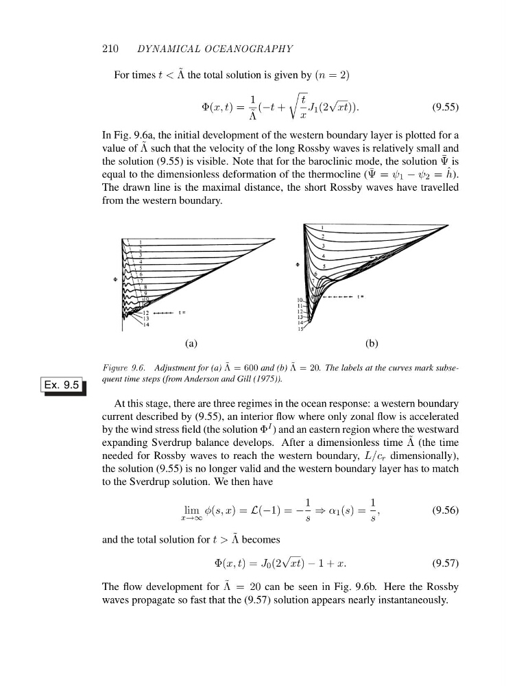
In Fig. 9.6a, the initial development of the western boundary layer is plotted for a
value of ˜
Λ such that the velocity of the long Rossby waves is relatively small and
the solution (9.55) is visible. Note that for the baroclinic mode, the solution ¯
Ψ is
equal to the dimensionless deformation of the thermocline ( ¯
Ψ=ψ 1 − ψ 2 = ˆ
h).
The drawn line is the maximal distance, the short Rossby waves have travelled
from the western boundary.
(a)
(b)
Figure 9.6. Adjustment for (a) ˜
Λ = 600 and (b) ˜
Λ=2 0 . The labels at the curves mark subsequent time steps (from Anderson and Gill (1975)).
Ex. 9.5
At this stage, there are three regimes in the ocean response: a western boundary
current described by (9.55), an interior flow where only zonal flow is accelerated
by the wind stress field (the solution Φ I ) and an eastern region where the westward
expanding Sverdrup balance develops. After a dimensionless time ˜
Λ (the time
needed for Rossby waves to reach the western boundary, L/c r dimensionally),
the solution (9.55) is no longer valid and the western boundary layer has to match
to the Sverdrup solution. We then have
lim
x→∞
φ(s, x)=L(−1) = −
1
s
⇒ α 1 (s)=
1
s
,
(9.56)
and the total solution for t> ˜
Λ becomes
Φ(x, t)=J 0 (2
√
xt) − 1+x.
(9.57)
The flow development for ˜
Λ=2 0can be seen in Fig. 9.6b. Here the Rossby
waves propagate so fast that the (9.57) solution appears nearly instantaneously.
DYNAMICAL OCEANOGRAPHY
For times t< ˜
Λ the total solution is given by (n =2)
Φ(x, t)=
1
˜
Λ
(−t +
t
x
J 1 (2
√
xt)).
(9.55)
In Fig. 9.6a, the initial development of the western boundary layer is plotted for a
value of ˜
Λ such that the velocity of the long Rossby waves is relatively small and
the solution (9.55) is visible. Note that for the baroclinic mode, the solution ¯
Ψ is
equal to the dimensionless deformation of the thermocline ( ¯
Ψ=ψ 1 − ψ 2 = ˆ
h).
The drawn line is the maximal distance, the short Rossby waves have travelled
from the western boundary.
(a)
(b)
Figure 9.6. Adjustment for (a) ˜
Λ = 600 and (b) ˜
Λ=2 0 . The labels at the curves mark subsequent time steps (from Anderson and Gill (1975)).
Ex. 9.5
At this stage, there are three regimes in the ocean response: a western boundary
current described by (9.55), an interior flow where only zonal flow is accelerated
by the wind stress field (the solution Φ I ) and an eastern region where the westward
expanding Sverdrup balance develops. After a dimensionless time ˜
Λ (the time
needed for Rossby waves to reach the western boundary, L/c r dimensionally),
the solution (9.55) is no longer valid and the western boundary layer has to match
to the Sverdrup solution. We then have
lim
x→∞
φ(s, x)=L(−1) = −
1
s
⇒ α 1 (s)=
1
s
,
(9.56)
and the total solution for t> ˜
Λ becomes
Φ(x, t)=J 0 (2
√
xt) − 1+x.
(9.57)
The flow development for ˜
Λ=2 0can be seen in Fig. 9.6b. Here the Rossby
waves propagate so fast that the (9.57) solution appears nearly instantaneously.