

204
DYNAMICAL OCEANOGRAPHY
x = 0
x = 1
y = 0
y = d
ψ = 0
ψ = 0
ψ = 0
ψ = 0
τ
x
τ
x
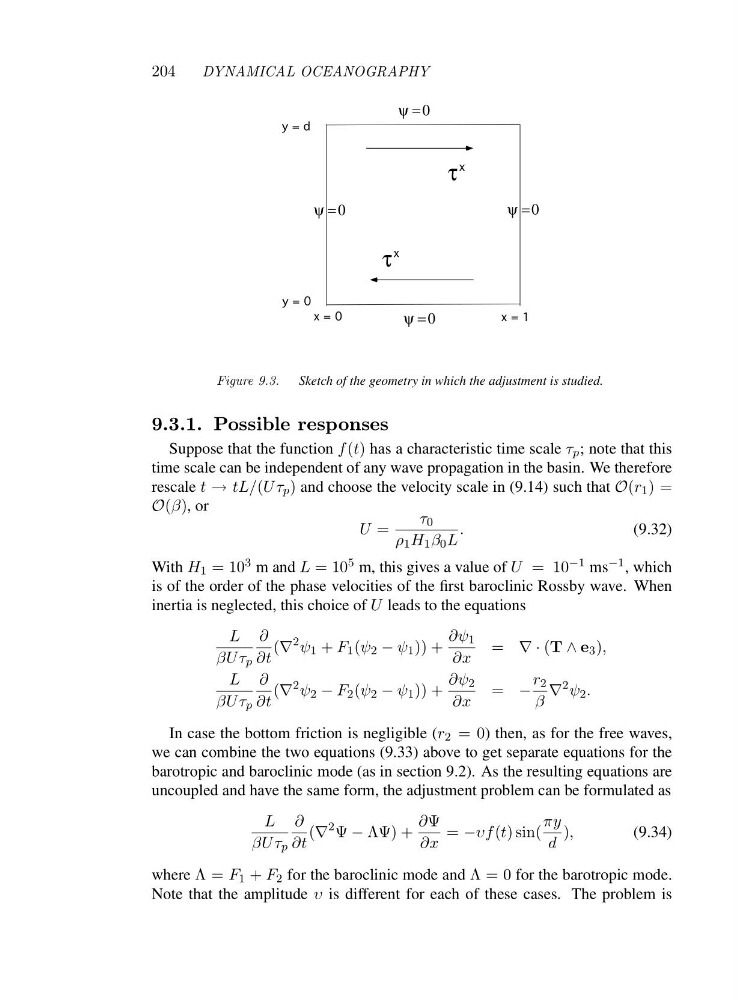
Figure 9.3. Sketch of the geometry in which the adjustment is studied.
9.3.1. Possible responses
Suppose that the function f (t) has a characteristic time scale τ p ; note that this
time scale can be independent of any wave propagation in the basin. We therefore
rescale t → tL/(Uτ p ) and choose the velocity scale in (9.14) such that O(r 1 )=
O(β),or
U =
τ 0
ρ 1 H 1 β 0 L
.
(9.32)
With H 1 =10 3 mandL =10 5 m, this gives a value of U =1 0 −1 ms −1 , which
is of the order of the phase velocities of the first baroclinic Rossby wave. When
inertia is neglected, this choice of U leads to the equations
L
βUτ p
∂
∂t
(∇
2 ψ 1 + F 1 (ψ 2 − ψ 1 )) +
∂ψ 1
∂x
= ∇·(T ∧ e 3 ),
L
βUτ p
∂
∂t
(∇
2 ψ 2 − F 2 (ψ 2 − ψ 1 )) +
∂ψ 2
∂x
= −
r 2
β
∇
2 ψ 2 .
In case the bottom friction is negligible (r 2 =0 ) then, as for the free waves,
we can combine the two equations (9.33) above to get separate equations for the
barotropic and baroclinic mode (as in section 9.2). As the resulting equations are
uncoupled and have the same form, the adjustment problem can be formulated as
L
βUτ p
∂
∂t
(∇
2 Ψ − ΛΨ) +
∂Ψ
∂x
= −υf(t)sin(
πy
d
),
(9.34)
where Λ=F 1 + F 2 for the baroclinic mode and Λ=0for the barotropic mode.
Note that the amplitude υ is different for each of these cases. The problem is
DYNAMICAL OCEANOGRAPHY
x = 0
x = 1
y = 0
y = d
ψ = 0
ψ = 0
ψ = 0
ψ = 0
τ
x
τ
x
Figure 9.3. Sketch of the geometry in which the adjustment is studied.
9.3.1. Possible responses
Suppose that the function f (t) has a characteristic time scale τ p ; note that this
time scale can be independent of any wave propagation in the basin. We therefore
rescale t → tL/(Uτ p ) and choose the velocity scale in (9.14) such that O(r 1 )=
O(β),or
U =
τ 0
ρ 1 H 1 β 0 L
.
(9.32)
With H 1 =10 3 mandL =10 5 m, this gives a value of U =1 0 −1 ms −1 , which
is of the order of the phase velocities of the first baroclinic Rossby wave. When
inertia is neglected, this choice of U leads to the equations
L
βUτ p
∂
∂t
(∇
2 ψ 1 + F 1 (ψ 2 − ψ 1 )) +
∂ψ 1
∂x
= ∇·(T ∧ e 3 ),
L
βUτ p
∂
∂t
(∇
2 ψ 2 − F 2 (ψ 2 − ψ 1 )) +
∂ψ 2
∂x
= −
r 2
β
∇
2 ψ 2 .
In case the bottom friction is negligible (r 2 =0 ) then, as for the free waves,
we can combine the two equations (9.33) above to get separate equations for the
barotropic and baroclinic mode (as in section 9.2). As the resulting equations are
uncoupled and have the same form, the adjustment problem can be formulated as
L
βUτ p
∂
∂t
(∇
2 Ψ − ΛΨ) +
∂Ψ
∂x
= −υf(t)sin(
πy
d
),
(9.34)
where Λ=F 1 + F 2 for the baroclinic mode and Λ=0for the barotropic mode.
Note that the amplitude υ is different for each of these cases. The problem is