

184
DYNAMICAL OCEANOGRAPHY
If there is again an O(ǫ) bottom topography, as in (5.70), with associated
boundary conditions (5.71), then the boundary condition for ψ at z = −1 becomes
w
1 =
1
S
(
∂
∂t
+ u
0 ∂
∂x
+ v
0 ∂
∂y
)
∂ψ
∂z
= u
0 .∇η b −
r
2
ζ
0 .
(8.33)
At the ocean-atmosphere interface it can also be shown that if E V ≪ ǫS,t h e
results of the homogeneous theory can also be used. The equation (5.77) (with
F = O(ǫ)), with (8.28), then gives the boundary condition at z =0
w
1 = −
1
S
(
∂
∂t
+ u
0 ∂
∂x
+ v
0 ∂
∂y
)
∂ψ
∂z
=
αr
2
∇.(T ∧ e 3 ),
(8.34)
where r is the parameter in (5.86), i.e. r = ¯
E
1/2
V /ǫ.
Because F = O(ǫ) and S = O(1), the deformation of the ocean-atmosphere
interface does not play any role in the stratified dynamics on the scale of the
Rossby deformation radius. The isopycnals deform much easier than the oceanatmosphere interface and those contribute most to the vorticity balance. For F =
O(ǫ), the ocean-atmosphere interface can be treated as a non-deformable surface;
this is called the ‘rigid lid’ approximation.
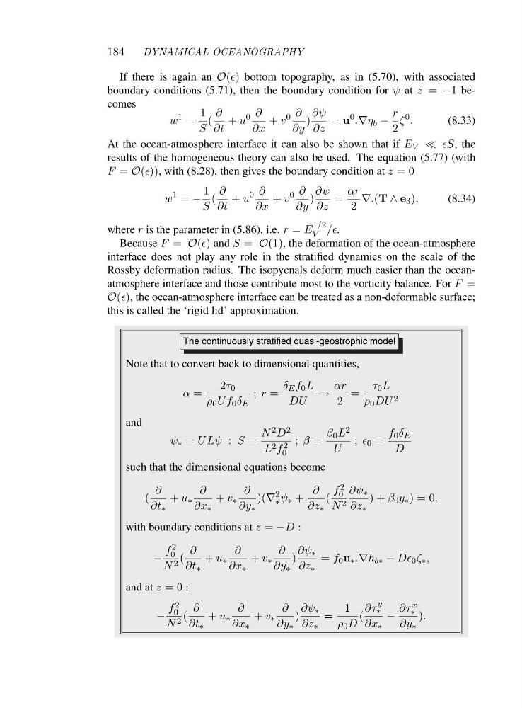
The continuously stratified quasi-geostrophic model
Note that to convert back to dimensional quantities,
α =
2τ 0
ρ 0 Uf 0 δ E
; r =
δ E f 0 L
DU
→
αr
2
=
τ 0 L
ρ 0 DU 2
and
ψ ∗ = ULψ : S =
N 2 D 2
L 2 f 2
0
; β =
β 0 L 2
U
; ǫ 0 =
f 0 δ E
D
such that the dimensional equations become
(
∂
∂t ∗
+ u ∗
∂
∂x ∗
+ v ∗
∂
∂y ∗
)(∇
2
∗ ψ ∗ +
∂
∂z ∗
(
f 2
0
N 2
∂ψ ∗
∂z ∗
)+β 0 y ∗ )=0,
with boundary conditions at z = −D :
−
f 2
0
N 2 (
∂
∂t ∗
+ u ∗
∂
∂x ∗
+ v ∗
∂
∂y ∗
)
∂ψ ∗
∂z ∗
= f 0 u ∗ .∇h b∗ − Dǫ 0 ζ ∗ ,
and at z =0:
−
f 2
0
N 2 (
∂
∂t ∗
+ u ∗
∂
∂x ∗
+ v ∗
∂
∂y ∗
)
∂ψ ∗
∂z ∗
=
1
ρ 0 D
(
∂τ
y
∗
∂x ∗
−
∂τ x
∗
∂y ∗
).
DYNAMICAL OCEANOGRAPHY
If there is again an O(ǫ) bottom topography, as in (5.70), with associated
boundary conditions (5.71), then the boundary condition for ψ at z = −1 becomes
w
1 =
1
S
(
∂
∂t
+ u
0 ∂
∂x
+ v
0 ∂
∂y
)
∂ψ
∂z
= u
0 .∇η b −
r
2
ζ
0 .
(8.33)
At the ocean-atmosphere interface it can also be shown that if E V ≪ ǫS,t h e
results of the homogeneous theory can also be used. The equation (5.77) (with
F = O(ǫ)), with (8.28), then gives the boundary condition at z =0
w
1 = −
1
S
(
∂
∂t
+ u
0 ∂
∂x
+ v
0 ∂
∂y
)
∂ψ
∂z
=
αr
2
∇.(T ∧ e 3 ),
(8.34)
where r is the parameter in (5.86), i.e. r = ¯
E
1/2
V /ǫ.
Because F = O(ǫ) and S = O(1), the deformation of the ocean-atmosphere
interface does not play any role in the stratified dynamics on the scale of the
Rossby deformation radius. The isopycnals deform much easier than the oceanatmosphere interface and those contribute most to the vorticity balance. For F =
O(ǫ), the ocean-atmosphere interface can be treated as a non-deformable surface;
this is called the ‘rigid lid’ approximation.
The continuously stratified quasi-geostrophic model
Note that to convert back to dimensional quantities,
α =
2τ 0
ρ 0 Uf 0 δ E
; r =
δ E f 0 L
DU
→
αr
2
=
τ 0 L
ρ 0 DU 2
and
ψ ∗ = ULψ : S =
N 2 D 2
L 2 f 2
0
; β =
β 0 L 2
U
; ǫ 0 =
f 0 δ E
D
such that the dimensional equations become
(
∂
∂t ∗
+ u ∗
∂
∂x ∗
+ v ∗
∂
∂y ∗
)(∇
2
∗ ψ ∗ +
∂
∂z ∗
(
f 2
0
N 2
∂ψ ∗
∂z ∗
)+β 0 y ∗ )=0,
with boundary conditions at z = −D :
−
f 2
0
N 2 (
∂
∂t ∗
+ u ∗
∂
∂x ∗
+ v ∗
∂
∂y ∗
)
∂ψ ∗
∂z ∗
= f 0 u ∗ .∇h b∗ − Dǫ 0 ζ ∗ ,
and at z =0:
−
f 2
0
N 2 (
∂
∂t ∗
+ u ∗
∂
∂x ∗
+ v ∗
∂
∂y ∗
)
∂ψ ∗
∂z ∗
=
1
ρ 0 D
(
∂τ
y
∗
∂x ∗
−
∂τ x
∗
∂y ∗
).