

138
DYNAMICAL OCEANOGRAPHY
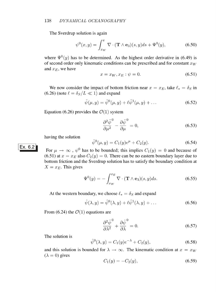
The Sverdrup solution is again
ψ
0 (x, y)=
x
x W
∇·(T ∧ e 3 )(s, y)ds +Ψ
0 (y),
(6.50)
where Ψ 0 (y) has to be determined. As the highest order derivative in (6.49) is
of second order only kinematic conditions can be prescribed and for constant x W
and x E ,wehave
x = x W ,x E : ψ =0.
(6.51)
We now consider the impact of bottom friction near x = x E ,tak eℓ ∗ = δ S in
(6.26) (note ℓ = δ S /L ≪ 1) and expand
˜
ψ(μ, y)= ˜
ψ
0 (μ, y)+ℓ ˜
ψ
1 (μ, y)+...
(6.52)
Equation (6.26) provides the O(1) system
∂ 2 ˜
ψ
∂μ 2
0
−
∂ ˜
ψ
∂μ
0
=0,
(6.53)
having the solution
˜
ψ
0 (μ, y)=C 1 (y)e
μ + C 2 (y).
(6.54)
For μ →∞, ψ 0 has to be bounded; this implies C 1 (y)=0and because of
Ex. 6.2
(6.51) at x = x E also C 2 (y)=0 . There can be no eastern boundary layer due to
bottom friction and the Sverdrup solution has to satisfy the boundary condition at
X = x E .T h i sg i v e s
Ψ
0 (y)=−
x E
x W
∇·(T ∧ e 3 )(s, y)ds.
(6.55)
At the western boundary, we choose ℓ ∗ = δ S and expand
ˆ
ψ(λ, y)= ˆ
ψ
0 (λ, y)+ℓ ˆ
ψ
1 (λ, y)+...
(6.56)
From (6.24) the O(1) equations are
∂ 2 ˆ
ψ
∂λ 2
0
+
∂ ˆ
ψ
∂λ
0
=0.
(6.57)
The solution is
ˆ
ψ
0 (λ, y)=C 1 (y)e
−λ + C 2 (y),
(6.58)
and this solution is bounded for λ →∞ . The kinematic condition at x = x W
(λ =0)gives
C 1 (y)=−C 2 (y),
(6.59)
DYNAMICAL OCEANOGRAPHY
The Sverdrup solution is again
ψ
0 (x, y)=
x
x W
∇·(T ∧ e 3 )(s, y)ds +Ψ
0 (y),
(6.50)
where Ψ 0 (y) has to be determined. As the highest order derivative in (6.49) is
of second order only kinematic conditions can be prescribed and for constant x W
and x E ,wehave
x = x W ,x E : ψ =0.
(6.51)
We now consider the impact of bottom friction near x = x E ,tak eℓ ∗ = δ S in
(6.26) (note ℓ = δ S /L ≪ 1) and expand
˜
ψ(μ, y)= ˜
ψ
0 (μ, y)+ℓ ˜
ψ
1 (μ, y)+...
(6.52)
Equation (6.26) provides the O(1) system
∂ 2 ˜
ψ
∂μ 2
0
−
∂ ˜
ψ
∂μ
0
=0,
(6.53)
having the solution
˜
ψ
0 (μ, y)=C 1 (y)e
μ + C 2 (y).
(6.54)
For μ →∞, ψ 0 has to be bounded; this implies C 1 (y)=0and because of
Ex. 6.2
(6.51) at x = x E also C 2 (y)=0 . There can be no eastern boundary layer due to
bottom friction and the Sverdrup solution has to satisfy the boundary condition at
X = x E .T h i sg i v e s
Ψ
0 (y)=−
x E
x W
∇·(T ∧ e 3 )(s, y)ds.
(6.55)
At the western boundary, we choose ℓ ∗ = δ S and expand
ˆ
ψ(λ, y)= ˆ
ψ
0 (λ, y)+ℓ ˆ
ψ
1 (λ, y)+...
(6.56)
From (6.24) the O(1) equations are
∂ 2 ˆ
ψ
∂λ 2
0
+
∂ ˆ
ψ
∂λ
0
=0.
(6.57)
The solution is
ˆ
ψ
0 (λ, y)=C 1 (y)e
−λ + C 2 (y),
(6.58)
and this solution is bounded for λ →∞ . The kinematic condition at x = x W
(λ =0)gives
C 1 (y)=−C 2 (y),
(6.59)