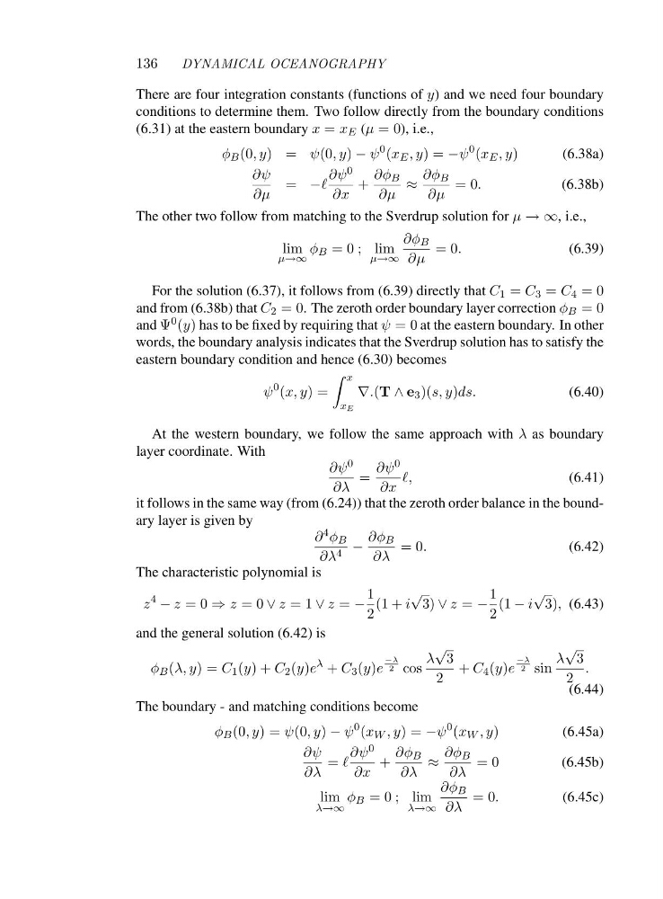
136
DYNAMICAL OCEANOGRAPHY
There are four integration constants (functions of y) and we need four boundary
conditions to determine them. Two follow directly from the boundary conditions
(6.31) at the eastern boundary x = x E (μ =0), i.e.,
φ B (0,y)=ψ(0,y) − ψ
0 (x E ,y)=−ψ
0 (x E ,y)
(6.38a)
∂ψ
∂μ
= −ℓ
∂ψ 0
∂x
+
∂φ B
∂μ
≈
∂φ B
∂μ
=0.
(6.38b)
The other two follow from matching to the Sverdrup solution for μ →∞, i.e.,
lim
μ→∞
φ B = 0 ; lim
μ→∞
∂φ B
∂μ
=0.
(6.39)
For the solution (6.37), it follows from (6.39) directly that C 1 = C 3 = C 4 =0
and from (6.38b) that C 2 =0. The zeroth order boundary layer correction φ B =0
and Ψ 0 (y) has to be fixed by requiring that ψ =0at the eastern boundary. In other
words, the boundary analysis indicates that the Sverdrup solution has to satisfy the
eastern boundary condition and hence (6.30) becomes
ψ
0 (x, y)=
x
x E
∇.(T ∧ e 3 )(s, y)ds.
(6.40)
At the western boundary, we follow the same approach with λ as boundary
layer coordinate. With
∂ψ 0
∂λ
=
∂ψ 0
∂x
ℓ,
(6.41)
it follows in the same way (from (6.24)) that the zeroth order balance in the boundary layer is given by
∂ 4 φ B
∂λ 4 −
∂φ B
∂λ
=0.
(6.42)
The characteristic polynomial is
z
4 − z =0⇒ z =0∨ z =1∨ z = −
1
2
(1 + i
√
3) ∨ z = −
1
2
(1 − i
√
3), (6.43)
and the general solution (6.42) is
φ B (λ, y)=C 1 (y)+C 2 (y)e
λ + C 3 (y)e
−λ
2 cos
λ
√
3
2
+ C 4 (y)e
−λ
2 sin
λ
√
3
2
.
(6.44)
The boundary - and matching conditions become
φ B (0,y)=ψ(0,y) − ψ
0 (x W ,y)=−ψ
0 (x W ,y)
(6.45a)
∂ψ
∂λ
= ℓ
∂ψ 0
∂x
+
∂φ B
∂λ
≈
∂φ B
∂λ
=0
(6.45b)
lim
λ→∞
φ B = 0 ; lim
λ→∞
∂φ B
∂λ
=0.
(6.45c)