

Wind-driven circulation
113
U
H
L
Δ
p
C
-
a
x
y
(a)
H
L
Δ
p
v
-
a
a
f
c
x
y
(b)
Figure 5.10. (a) Geostrophic balance outside the bottom Ekman boundary layer: the pressure
gradient ∇p balances the Coriolis acceleration a
c (hence the sum of a
c and −∇p is zero). (b)
Balance in the Ekman boundary layer, where the sum of the Coriolis acceleration and the frictional
acceleration a
f compensate the pressure gradient.
◭
5.3.4. Continuity of the vertical velocity
The results so far of the outer geostrophic flow and the inner Ekman boundary
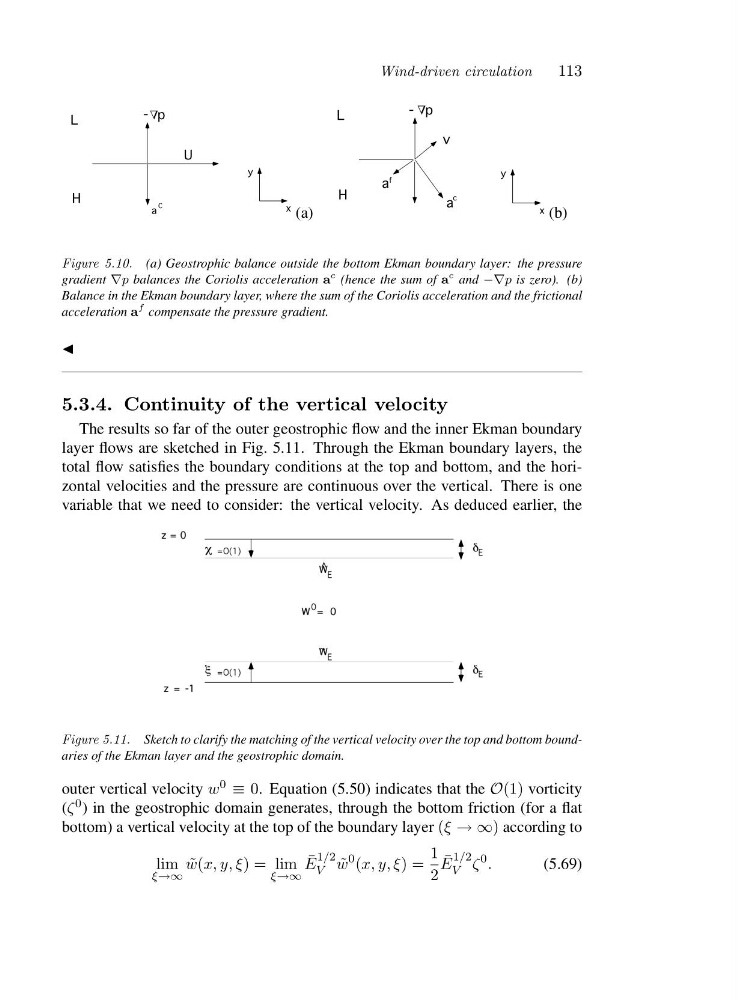
layer flows are sketched in Fig. 5.11. Through the Ekman boundary layers, the
total flow satisfies the boundary conditions at the top and bottom, and the horizontal velocities and the pressure are continuous over the vertical. There is one
variable that we need to consider: the vertical velocity. As deduced earlier, the
Figure 5.11. Sketch to clarify the matching of the vertical velocity over the top and bottom boundaries of the Ekman layer and the geostrophic domain.
outer vertical velocity w 0 ≡ 0. Equation (5.50) indicates that the O(1) vorticity
(ζ 0 ) in the geostrophic domain generates, through the bottom friction (for a flat
bottom) a vertical velocity at the top of the boundary layer (ξ →∞) according to
lim
ξ→∞
˜
w(x, y, ξ) = lim
ξ→∞
¯
E
1/2
V ˜
w
0 (x, y, ξ)=
1
2
¯
E
1/2
V ζ
0 .
(5.69)
113
U
H
L
Δ
p
C
-
a
x
y
(a)
H
L
Δ
p
v
-
a
a
f
c
x
y
(b)
Figure 5.10. (a) Geostrophic balance outside the bottom Ekman boundary layer: the pressure
gradient ∇p balances the Coriolis acceleration a
c (hence the sum of a
c and −∇p is zero). (b)
Balance in the Ekman boundary layer, where the sum of the Coriolis acceleration and the frictional
acceleration a
f compensate the pressure gradient.
◭
5.3.4. Continuity of the vertical velocity
The results so far of the outer geostrophic flow and the inner Ekman boundary
layer flows are sketched in Fig. 5.11. Through the Ekman boundary layers, the
total flow satisfies the boundary conditions at the top and bottom, and the horizontal velocities and the pressure are continuous over the vertical. There is one
variable that we need to consider: the vertical velocity. As deduced earlier, the
Figure 5.11. Sketch to clarify the matching of the vertical velocity over the top and bottom boundaries of the Ekman layer and the geostrophic domain.
outer vertical velocity w 0 ≡ 0. Equation (5.50) indicates that the O(1) vorticity
(ζ 0 ) in the geostrophic domain generates, through the bottom friction (for a flat
bottom) a vertical velocity at the top of the boundary layer (ξ →∞) according to
lim
ξ→∞
˜
w(x, y, ξ) = lim
ξ→∞
¯
E
1/2
V ˜
w
0 (x, y, ξ)=
1
2
¯
E
1/2
V ζ
0 .
(5.69)