

96
DYNAMICAL OCEANOGRAPHY
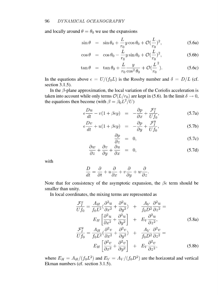
and locally around θ = θ 0 we use the expansions
sin θ =s i n θ 0 +
L
r 0
y cos θ 0 + O(
L
r 0
)
2 ,
(5.6a)
cos θ =c o s θ 0 −
L
r 0
y sin θ 0 + O(
L
r 0
)
2 ,
(5.6b)
tan θ =t a n θ 0 +
L
r 0
y
cos 2 θ 0
+ O(
L
r 0
2
).
(5.6c)
In the equations above ǫ = U/(f 0 L) is the Rossby number and δ = D/L (cf.
section 3.1.5).
In the β-plane approximation, the local variation of the Coriolis acceleration is
taken into account while only terms O(L/r 0 ) are kept in (5.6). In the limit δ → 0,
the equations then become (with β = β 0 L 2 /U )
ǫ
Du
dt
− v(1 + βǫy)=−
∂p
∂x
+
F x
I
Uf 0
,
(5.7a)
ǫ
Dv
dt
+ u(1 + βǫy)=−
∂p
∂y
+
F
y
I
Uf 0
,
(5.7b)
∂p
∂z
=0 ,
(5.7c)
∂w
∂z
+
∂v
∂y
+
∂u
∂x
=0 ,
(5.7d)
with
D
dt
=
∂
∂t
+ u
∂
∂x
+ v
∂
∂y
+ w
∂
∂z
.
Note that for consistency of the asymptotic expansion, the βǫ term should be
smaller than unity.
In local coordinates, the mixing terms are represented as
F x
I
Uf 0
=
A H
f 0 L 2 (
∂ 2 u
∂x 2 +
∂ 2 u
∂y 2 )+
A V
f 0 D 2
∂ 2 u
∂z 2 =
E H
∂ 2 u
∂x 2 +
∂ 2 u
∂y 2
+ E V
∂ 2 u
∂z 2 ,
(5.8a)
F
y
I
Uf 0
=
A H
f 0 L 2 (
∂ 2 v
∂x 2 +
∂ 2 v
∂y 2 )+
A V
f 0 D 2
∂ 2 v
∂z 2 =
E H
∂ 2 v
∂x 2 +
∂ 2 v
∂y 2
+ E V
∂ 2 v
∂z 2 ,
(5.8b)
where E H = A H /(f 0 L 2 ) and E V = A V /(f 0 D 2 ) are the horizontal and vertical
Ekman numbers (cf. section 3.1.5).
DYNAMICAL OCEANOGRAPHY
and locally around θ = θ 0 we use the expansions
sin θ =s i n θ 0 +
L
r 0
y cos θ 0 + O(
L
r 0
)
2 ,
(5.6a)
cos θ =c o s θ 0 −
L
r 0
y sin θ 0 + O(
L
r 0
)
2 ,
(5.6b)
tan θ =t a n θ 0 +
L
r 0
y
cos 2 θ 0
+ O(
L
r 0
2
).
(5.6c)
In the equations above ǫ = U/(f 0 L) is the Rossby number and δ = D/L (cf.
section 3.1.5).
In the β-plane approximation, the local variation of the Coriolis acceleration is
taken into account while only terms O(L/r 0 ) are kept in (5.6). In the limit δ → 0,
the equations then become (with β = β 0 L 2 /U )
ǫ
Du
dt
− v(1 + βǫy)=−
∂p
∂x
+
F x
I
Uf 0
,
(5.7a)
ǫ
Dv
dt
+ u(1 + βǫy)=−
∂p
∂y
+
F
y
I
Uf 0
,
(5.7b)
∂p
∂z
=0 ,
(5.7c)
∂w
∂z
+
∂v
∂y
+
∂u
∂x
=0 ,
(5.7d)
with
D
dt
=
∂
∂t
+ u
∂
∂x
+ v
∂
∂y
+ w
∂
∂z
.
Note that for consistency of the asymptotic expansion, the βǫ term should be
smaller than unity.
In local coordinates, the mixing terms are represented as
F x
I
Uf 0
=
A H
f 0 L 2 (
∂ 2 u
∂x 2 +
∂ 2 u
∂y 2 )+
A V
f 0 D 2
∂ 2 u
∂z 2 =
E H
∂ 2 u
∂x 2 +
∂ 2 u
∂y 2
+ E V
∂ 2 u
∂z 2 ,
(5.8a)
F
y
I
Uf 0
=
A H
f 0 L 2 (
∂ 2 v
∂x 2 +
∂ 2 v
∂y 2 )+
A V
f 0 D 2
∂ 2 v
∂z 2 =
E H
∂ 2 v
∂x 2 +
∂ 2 v
∂y 2
+ E V
∂ 2 v
∂z 2 ,
(5.8b)
where E H = A H /(f 0 L 2 ) and E V = A V /(f 0 D 2 ) are the horizontal and vertical
Ekman numbers (cf. section 3.1.5).