

Internal Solitary Waves in a Layered Weakly Stratified Flow
59
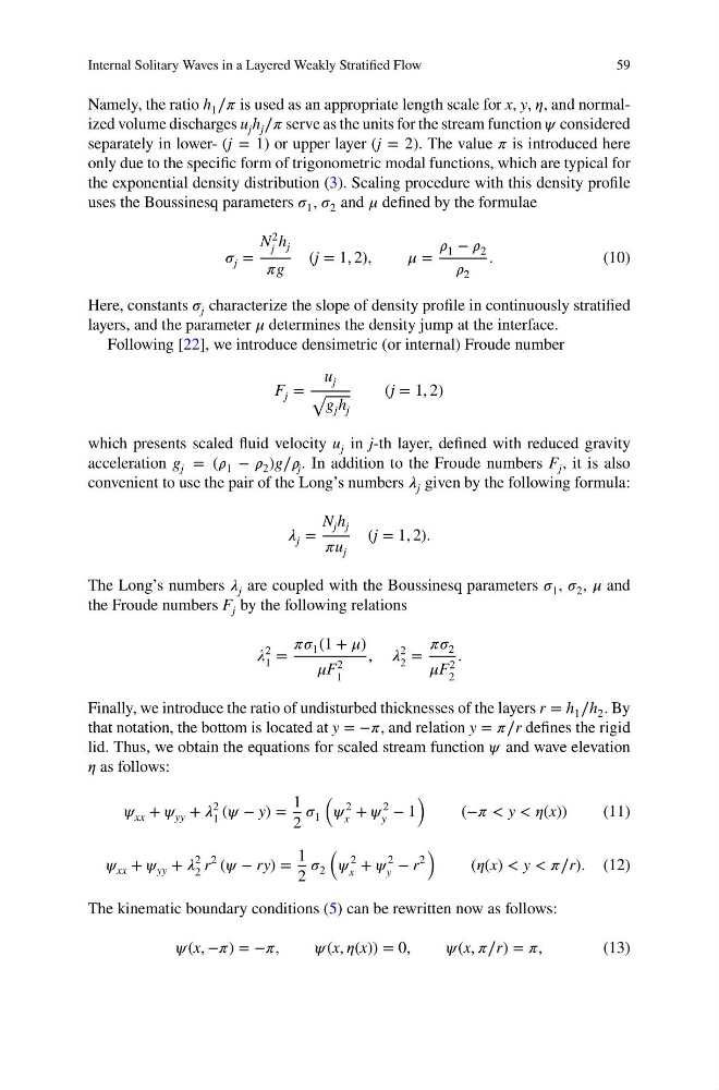
Namely, the ratio h 1 ∕í µí¼ is used as an appropriate length scale for x, y, í µí¼, and normalized volume discharges u j h j ∕í µí¼ serve as the units for the stream function í µí¼ considered
separately in lower- (j = 1) or upper layer (j = 2). The value í µí¼ is introduced here
only due to the specific form of trigonometric modal functions, which are typical for
the exponential density distribution (3). Scaling procedure with this density profile
uses the Boussinesq parameters í µí¼ 1 , í µí¼ 2 and í µí¼ defined by the formulae
í µí¼ j =
N
2
j
h j
í µí¼g
(j = 1, 2),
í µí¼=
í µí¼ 1 − í µí¼ 2
í µí¼ 2
.
(10)
Here, constants í µí¼ j characterize the slope of density profile in continuously stratified
layers, and the parameter í µí¼ determines the density jump at the interface.
Following [22], we introduce densimetric (or internal) Froude number
F j =
u j
√
g j h j
(j = 1, 2)
which presents scaled fluid velocity u j in j-th layer, defined with reduced gravity
acceleration g j = (í µí¼ 1 − í µí¼ 2 )g∕í µí¼ j . In addition to the Froude numbers F j , it is also
convenient to use the pair of the Long’s numbers í µí¼ j given by the following formula:
í µí¼ j =
N j h j
í µí¼u j
(j = 1, 2).
The Long’s numbers í µí¼ j are coupled with the Boussinesq parameters í µí¼ 1 , í µí¼ 2 , í µí¼ and
the Froude numbers F j by the following relations
í µí¼
2
1
=
í µí¼í µí¼ 1 (1 + í µí¼)
í µí¼F
2
1
, í µí¼
2
2
=
í µí¼í µí¼ 2
í µí¼F
2
2
.
Finally, we introduce the ratio of undisturbed thicknesses of the layers r = h 1 ∕h 2 . By
that notation, the bottom is located at y = −í µí¼, and relation y = í µí¼∕r defines the rigid
lid. Thus, we obtain the equations for scaled stream function í µí¼ and wave elevation
í µí¼ as follows:
í µí¼ xx + í µí¼ yy + í µí¼
2
1
(í µí¼ − y) =
1
2
í µí¼ 1
(
í µí¼
2
x
+ í µí¼
2
y
− 1
)
(−í µí¼ < y < í µí¼(x))
(11)
í µí¼ xx + í µí¼ yy + í µí¼
2
2
r
2
(í µí¼ − ry) =
1
2
í µí¼ 2
(
í µí¼
2
x
+ í µí¼
2
y
− r
2
)
(í µí¼(x) < y < í µí¼∕r). (12)
The kinematic boundary conditions (5) can be rewritten now as follows:
í µí¼(x, −í µí¼) = −í µí¼,
í µí¼(x, í µí¼(x)) = 0,
í µí¼(x, í µí¼∕r) = í µí¼,
(13)
59
Namely, the ratio h 1 ∕í µí¼ is used as an appropriate length scale for x, y, í µí¼, and normalized volume discharges u j h j ∕í µí¼ serve as the units for the stream function í µí¼ considered
separately in lower- (j = 1) or upper layer (j = 2). The value í µí¼ is introduced here
only due to the specific form of trigonometric modal functions, which are typical for
the exponential density distribution (3). Scaling procedure with this density profile
uses the Boussinesq parameters í µí¼ 1 , í µí¼ 2 and í µí¼ defined by the formulae
í µí¼ j =
N
2
j
h j
í µí¼g
(j = 1, 2),
í µí¼=
í µí¼ 1 − í µí¼ 2
í µí¼ 2
.
(10)
Here, constants í µí¼ j characterize the slope of density profile in continuously stratified
layers, and the parameter í µí¼ determines the density jump at the interface.
Following [22], we introduce densimetric (or internal) Froude number
F j =
u j
√
g j h j
(j = 1, 2)
which presents scaled fluid velocity u j in j-th layer, defined with reduced gravity
acceleration g j = (í µí¼ 1 − í µí¼ 2 )g∕í µí¼ j . In addition to the Froude numbers F j , it is also
convenient to use the pair of the Long’s numbers í µí¼ j given by the following formula:
í µí¼ j =
N j h j
í µí¼u j
(j = 1, 2).
The Long’s numbers í µí¼ j are coupled with the Boussinesq parameters í µí¼ 1 , í µí¼ 2 , í µí¼ and
the Froude numbers F j by the following relations
í µí¼
2
1
=
í µí¼í µí¼ 1 (1 + í µí¼)
í µí¼F
2
1
, í µí¼
2
2
=
í µí¼í µí¼ 2
í µí¼F
2
2
.
Finally, we introduce the ratio of undisturbed thicknesses of the layers r = h 1 ∕h 2 . By
that notation, the bottom is located at y = −í µí¼, and relation y = í µí¼∕r defines the rigid
lid. Thus, we obtain the equations for scaled stream function í µí¼ and wave elevation
í µí¼ as follows:
í µí¼ xx + í µí¼ yy + í µí¼
2
1
(í µí¼ − y) =
1
2
í µí¼ 1
(
í µí¼
2
x
+ í µí¼
2
y
− 1
)
(−í µí¼ < y < í µí¼(x))
(11)
í µí¼ xx + í µí¼ yy + í µí¼
2
2
r
2
(í µí¼ − ry) =
1
2
í µí¼ 2
(
í µí¼
2
x
+ í µí¼
2
y
− r
2
)
(í µí¼(x) < y < í µí¼∕r). (12)
The kinematic boundary conditions (5) can be rewritten now as follows:
í µí¼(x, −í µí¼) = −í µí¼,
í µí¼(x, í µí¼(x)) = 0,
í µí¼(x, í µí¼∕r) = í µí¼,
(13)