

On the other hand, the recent modeling experience shows that the model ability
to reproduce observed phenomena depends on the spatial resolution, while it is
possibly controlled not by the resolution only [1]. It may be treated as the manifestation of the complex nonlinear physics of the ocean and sea ice, which should
be investigated more carefully.
Hydrostatic and Non-hydrostatic Ocean Dynamics
In order to look into the causes of the faults in the AO modeling it is worth recalling
the basics of the modern large-scale ocean models. Traditionally hydrostatic,
Boussinesq, and incompressibility (divu⃗ = 0) approximations are used. Apart of
them, the special form of equations is used in the so-called “shallow water
approximation” in the z-coordinate system, when “horizontal” motions at the surface normal to the sum of the local gravity+centrifugal acceleration (we denote
them by index h) and “vertical” ones in the direction of this sum, are specified. The
initial system of equations appears to be specified on the manifold called “cylinder
over sphere”. A series of simplifications has to be performed to ensure analogs of
energy and angular momentum conservation laws.
The common approach is to use the Boussinesq approximation with the constant
reference density ρ c . It may be done if the pressure in the state equation will be
redefined p → p 0 = ρ c gz: otherwise, the energy will be imbalanced [10]. Moreover,
if the deviations of density e and pressure p′ from the reference values ρ c , p 0 are
defined, then the system of equations of the ocean hydro thermodynamics (in the
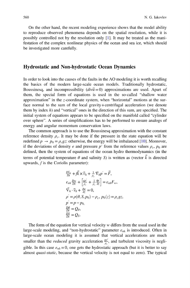
terms of potential temperature θ and salinity S) is written as (vector k ⃗ is directed
upwards, f is the Coriolis parameter):
Dv⃗ h
Dt + fk ⃗ × v⃗ h +
1
ρ c
∇⃗ h p
′ = F ⃗ ,
ε nh
Dw
Dt +
gρ
′
ρ c
+
1
ρ c
∂p
′
∂z
h
i
= ε nh F w ,
∇ ⃗
h ⋅ v⃗ h +
∂w
∂z = 0,
ρ
′ = ρ θ, S, p 0
ð
Þ− ρ c , p 0 ðzÞ = ρ c gz,
p
′ = p − p 0,
Dθ
Dt = Q θ ,
DS
Dt = Q S .
The form of the equation for vertical velocity w differs from the usual used in the
large-scale modeling, and “non-hydrostatic” parameter ε nh is introduced. Often in
large-scale ocean modeling it is assumed that vertical accelerations are much
smaller than the reduced gravity acceleration
gρ′
ρ c
, and turbulent viscosity is negligible. In this case ε nh = 0, one gets the hydrostatic approach (but it is better to say
almost quasi-static, because the vertical velocity is not equal to zero). The typical
560
N. G. Iakovlev
to reproduce observed phenomena depends on the spatial resolution, while it is
possibly controlled not by the resolution only [1]. It may be treated as the manifestation of the complex nonlinear physics of the ocean and sea ice, which should
be investigated more carefully.
Hydrostatic and Non-hydrostatic Ocean Dynamics
In order to look into the causes of the faults in the AO modeling it is worth recalling
the basics of the modern large-scale ocean models. Traditionally hydrostatic,
Boussinesq, and incompressibility (divu⃗ = 0) approximations are used. Apart of
them, the special form of equations is used in the so-called “shallow water
approximation” in the z-coordinate system, when “horizontal” motions at the surface normal to the sum of the local gravity+centrifugal acceleration (we denote
them by index h) and “vertical” ones in the direction of this sum, are specified. The
initial system of equations appears to be specified on the manifold called “cylinder
over sphere”. A series of simplifications has to be performed to ensure analogs of
energy and angular momentum conservation laws.
The common approach is to use the Boussinesq approximation with the constant
reference density ρ c . It may be done if the pressure in the state equation will be
redefined p → p 0 = ρ c gz: otherwise, the energy will be imbalanced [10]. Moreover,
if the deviations of density e and pressure p′ from the reference values ρ c , p 0 are
defined, then the system of equations of the ocean hydro thermodynamics (in the
terms of potential temperature θ and salinity S) is written as (vector k ⃗ is directed
upwards, f is the Coriolis parameter):
Dv⃗ h
Dt + fk ⃗ × v⃗ h +
1
ρ c
∇⃗ h p
′ = F ⃗ ,
ε nh
Dw
Dt +
gρ
′
ρ c
+
1
ρ c
∂p
′
∂z
h
i
= ε nh F w ,
∇ ⃗
h ⋅ v⃗ h +
∂w
∂z = 0,
ρ
′ = ρ θ, S, p 0
ð
Þ− ρ c , p 0 ðzÞ = ρ c gz,
p
′ = p − p 0,
Dθ
Dt = Q θ ,
DS
Dt = Q S .
The form of the equation for vertical velocity w differs from the usual used in the
large-scale modeling, and “non-hydrostatic” parameter ε nh is introduced. Often in
large-scale ocean modeling it is assumed that vertical accelerations are much
smaller than the reduced gravity acceleration
gρ′
ρ c
, and turbulent viscosity is negligible. In this case ε nh = 0, one gets the hydrostatic approach (but it is better to say
almost quasi-static, because the vertical velocity is not equal to zero). The typical
560
N. G. Iakovlev