

moments of the position of the measuring equipment at the bottom. The validity of
exactly this choice of points and moments of stations is considered in section “Error
Estimates” to estimate the errors. The calculation of the transport deviation Q t due to
the current non-stationarity and the non-simultaneity of hydrographic measurements
was performed at the midpoints of the spaces between the stations. The bottom relief
along the tracks of the sections necessary for estimating the transports was calculated
by linear interpolation from the nodes of the digital data array to the section line over
steps of approximately 0.1 km, so that the whole number of spaces between the station
points would be located between the station points. The results of all the calculations
are shown in Table 2 and in Figs. 4, 5, 6, 7, 8, 9, 10, 11, 12, 13, 14 and 15.
Error Estimates
Before proceeding to the analysis of the results of calculations it is necessary to
estimate their accuracy. It has two constituents: the accuracy of the data and the
accuracy of the calculation procedure.
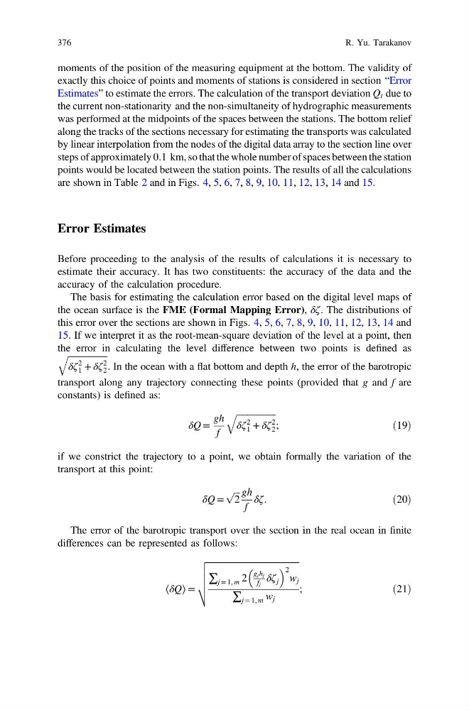
The basis for estimating the calculation error based on the digital level maps of
the ocean surface is the FME (Formal Mapping Error), δζ. The distributions of
this error over the sections are shown in Figs. 4, 5, 6, 7, 8, 9, 10, 11, 12, 13, 14 and
15. If we interpret it as the root-mean-square deviation of the level at a point, then
the error in calculating the level difference between two points is defined as
ffiffiffiffiffiffiffiffiffiffiffiffiffiffiffiffiffiffi
δζ
2
1 + δζ
2
2
q
. In the ocean with a flat bottom and depth h, the error of the barotropic
transport along any trajectory connecting these points (provided that g and f are
constants) is defined as:
δQ =
gh
f
ffiffiffiffiffiffiffiffiffiffiffiffiffiffiffiffiffiffi
δζ
2
1 + δζ
2
2
q
;
ð19Þ
if we constrict the trajectory to a point, we obtain formally the variation of the
transport at this point:
δQ =
ffiffi ffi
2
p gh
f
δζ.
ð20Þ
The error of the barotropic transport over the section in the real ocean in finite
differences can be represented as follows:
⟨δQ⟩ =
ffiffiffiffiffiffiffiffiffiffiffiffiffiffiffiffiffiffiffiffiffiffiffiffiffiffiffiffiffiffiffiffiffiffiffiffiffiffiffiffiffi ffi
∑ j = 1, m 2
g j h j
f j
δζ j
2
w j
∑ j = 1, m w j
v
u
u
u
t
;
ð21Þ
376
R. Yu. Tarakanov
exactly this choice of points and moments of stations is considered in section “Error
Estimates” to estimate the errors. The calculation of the transport deviation Q t due to
the current non-stationarity and the non-simultaneity of hydrographic measurements
was performed at the midpoints of the spaces between the stations. The bottom relief
along the tracks of the sections necessary for estimating the transports was calculated
by linear interpolation from the nodes of the digital data array to the section line over
steps of approximately 0.1 km, so that the whole number of spaces between the station
points would be located between the station points. The results of all the calculations
are shown in Table 2 and in Figs. 4, 5, 6, 7, 8, 9, 10, 11, 12, 13, 14 and 15.
Error Estimates
Before proceeding to the analysis of the results of calculations it is necessary to
estimate their accuracy. It has two constituents: the accuracy of the data and the
accuracy of the calculation procedure.
The basis for estimating the calculation error based on the digital level maps of
the ocean surface is the FME (Formal Mapping Error), δζ. The distributions of
this error over the sections are shown in Figs. 4, 5, 6, 7, 8, 9, 10, 11, 12, 13, 14 and
15. If we interpret it as the root-mean-square deviation of the level at a point, then
the error in calculating the level difference between two points is defined as
ffiffiffiffiffiffiffiffiffiffiffiffiffiffiffiffiffiffi
δζ
2
1 + δζ
2
2
q
. In the ocean with a flat bottom and depth h, the error of the barotropic
transport along any trajectory connecting these points (provided that g and f are
constants) is defined as:
δQ =
gh
f
ffiffiffiffiffiffiffiffiffiffiffiffiffiffiffiffiffiffi
δζ
2
1 + δζ
2
2
q
;
ð19Þ
if we constrict the trajectory to a point, we obtain formally the variation of the
transport at this point:
δQ =
ffiffi ffi
2
p gh
f
δζ.
ð20Þ
The error of the barotropic transport over the section in the real ocean in finite
differences can be represented as follows:
⟨δQ⟩ =
ffiffiffiffiffiffiffiffiffiffiffiffiffiffiffiffiffiffiffiffiffiffiffiffiffiffiffiffiffiffiffiffiffiffiffiffiffiffiffiffiffi ffi
∑ j = 1, m 2
g j h j
f j
δζ j
2
w j
∑ j = 1, m w j
v
u
u
u
t
;
ð21Þ
376
R. Yu. Tarakanov