

Internal Undular Bores in the Coastal Ocean
25
í µí¼ =
í µí¼
c
, í µí»¿ =
í µí¼
c 3 .
(11)
A further simplification is to absorb the factor Q,
U = Q
1∕2
í µí¼ , U T +
í µí¼
Q 1∕2 UU X + í µí»¿U XXX + í µí¼U = 0 .
(12)
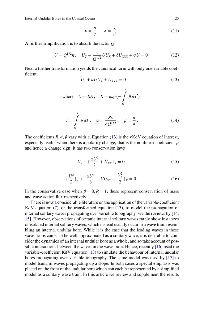
Next a further transformation yields the canonical form with only one variable coefficient,
U í µí¼ + í µí»¼UU X + U XXX = 0 ,
(13)
where U = RA , R = exp (−
í µí¼
∫
0
í µí»½ dí µí¼
′
) ,
í µí¼ =
T
∫
0
í µí»¿ dT , í µí»¼ =
Rí µí¼
í µí»¿Q 1∕2 , í µí»½ =
í µí¼
í µí»¿
.
(14)
The coefficients R, í µí»¼, í µí»½ vary with í µí¼. Equation (13) is the vKdV equation of interest,
especially useful when there is a polarity change, that is the nonlinear coefficient í µí¼
and hence í µí»¼ change sign. It has two conservation laws
U í µí¼ + {
í µí»¼U 2
2
+ U XX } X = 0 ,
(15)
{
U 2
2
} í µí¼ + {
í µí»¼U 3
3
+ UU XX −
U
2
X
2
} X = 0 .
(16)
In the conservative case when í µí»½ = 0, R = 1, these represent conservation of mass
and wave action flux respectively.
There is now a considerable literature on the application of the variable-coefficient
KdV equation (7), or the transformed equation (13), to model the propagation of
internal solitary waves propagating over variable topography, see the reviews by [14,
15]. However, observations of oceanic internal solitary waves rarely show instances
of isolated internal solitary waves, which instead usually occur in a wave train resembling an internal undular bore. While it is the case that the leading waves in these
wave trains can each be well approximated as a solitary wave, it is desirable to consider the dynamics of an internal undular bore as a whole, and so take account of possible interactions between the waves in the wave train. Hence, recently [16] used the
variable-coefficient KdV equation (13) to simulate the behaviour of internal undular
bores propagating over variable topography. The same model was used by [17] to
model tsunami waves propagating up a slope. In both cases a special emphasis was
placed on the front of the undular bore which can each be represented by a simplified
model as a solitary wave train. In this article we review and supplement the results
25
í µí¼ =
í µí¼
c
, í µí»¿ =
í µí¼
c 3 .
(11)
A further simplification is to absorb the factor Q,
U = Q
1∕2
í µí¼ , U T +
í µí¼
Q 1∕2 UU X + í µí»¿U XXX + í µí¼U = 0 .
(12)
Next a further transformation yields the canonical form with only one variable coefficient,
U í µí¼ + í µí»¼UU X + U XXX = 0 ,
(13)
where U = RA , R = exp (−
í µí¼
∫
0
í µí»½ dí µí¼
′
) ,
í µí¼ =
T
∫
0
í µí»¿ dT , í µí»¼ =
Rí µí¼
í µí»¿Q 1∕2 , í µí»½ =
í µí¼
í µí»¿
.
(14)
The coefficients R, í µí»¼, í µí»½ vary with í µí¼. Equation (13) is the vKdV equation of interest,
especially useful when there is a polarity change, that is the nonlinear coefficient í µí¼
and hence í µí»¼ change sign. It has two conservation laws
U í µí¼ + {
í µí»¼U 2
2
+ U XX } X = 0 ,
(15)
{
U 2
2
} í µí¼ + {
í µí»¼U 3
3
+ UU XX −
U
2
X
2
} X = 0 .
(16)
In the conservative case when í µí»½ = 0, R = 1, these represent conservation of mass
and wave action flux respectively.
There is now a considerable literature on the application of the variable-coefficient
KdV equation (7), or the transformed equation (13), to model the propagation of
internal solitary waves propagating over variable topography, see the reviews by [14,
15]. However, observations of oceanic internal solitary waves rarely show instances
of isolated internal solitary waves, which instead usually occur in a wave train resembling an internal undular bore. While it is the case that the leading waves in these
wave trains can each be well approximated as a solitary wave, it is desirable to consider the dynamics of an internal undular bore as a whole, and so take account of possible interactions between the waves in the wave train. Hence, recently [16] used the
variable-coefficient KdV equation (13) to simulate the behaviour of internal undular
bores propagating over variable topography. The same model was used by [17] to
model tsunami waves propagating up a slope. In both cases a special emphasis was
placed on the front of the undular bore which can each be represented by a simplified
model as a solitary wave train. In this article we review and supplement the results