

possible wave motion. The adjustment of stratified fluid where GWs co-exist with
internal waves is considered in section “Stably-Neutrally Stratified Fluid” using the
model of stably-neutrally stratified (SNS) fluid. The fluid consists of a stratified
upper layer with N > f and a homogeneous lower layer, the density and other fields
are continuous at the interface between the layers. The configuration is of practical
interest since recent observations indicate that, at least in some parts of the World
Ocean, there exist practically homogeneous or very weakly stratified (i.e. at N ≤ f )
near bottom layers several hundred meters thick [26, 27].
Both sections “Barotropic Model” and “Stably-Neutrally Stratified Fluid” are
organized similarly. In subsections “Governing Equations” the governing equations
with boundary and initial conditions are presented. In subsections “Linear Gyroscopic Waves” and “Linear Wave Modes” linear waves are discussed. The linear
invariants, geostrophic modes and linear adjustment are examined in subsections “Geostrophic Mode and Linear Adjustment” and “Invariants of Motion and
Geostrophic Mode”. In subsections “Non-dimensional Equations and Asymptotic
Solution” and “Non-dimensional Equations and the Lowest-Order Solution”
non-dimensional equations, an asymptotic procedure for finding the solution, and the
lowest-order solution are given. The slowly evolving components of motion (quasigeostrophic (QG) flow and inertial oscillations) are described in subsections “Slow
Evolution” and “Slow Evolution of the QG Component and Inertial Oscillations”.
Final section “Summary and Discussion” contains a discussion and conclusions.
Barotropic Model
Governing Equations
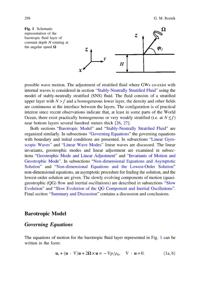
The equations of motion for the barotropic fluid layer represented in Fig. 1 can be
written in the form:
u t + ðu ⋅ ∇Þu + 2Ω × u = − ∇p ̸ ρ 0 , ∇ ⋅ u = 0.
ð1a; bÞ
Fig. 1 Schematic
representation of the
barotropic fluid layer of
constant depth H rotating at
the angular speed Ω
298
G. M. Reznik
internal waves is considered in section “Stably-Neutrally Stratified Fluid” using the
model of stably-neutrally stratified (SNS) fluid. The fluid consists of a stratified
upper layer with N > f and a homogeneous lower layer, the density and other fields
are continuous at the interface between the layers. The configuration is of practical
interest since recent observations indicate that, at least in some parts of the World
Ocean, there exist practically homogeneous or very weakly stratified (i.e. at N ≤ f )
near bottom layers several hundred meters thick [26, 27].
Both sections “Barotropic Model” and “Stably-Neutrally Stratified Fluid” are
organized similarly. In subsections “Governing Equations” the governing equations
with boundary and initial conditions are presented. In subsections “Linear Gyroscopic Waves” and “Linear Wave Modes” linear waves are discussed. The linear
invariants, geostrophic modes and linear adjustment are examined in subsections “Geostrophic Mode and Linear Adjustment” and “Invariants of Motion and
Geostrophic Mode”. In subsections “Non-dimensional Equations and Asymptotic
Solution” and “Non-dimensional Equations and the Lowest-Order Solution”
non-dimensional equations, an asymptotic procedure for finding the solution, and the
lowest-order solution are given. The slowly evolving components of motion (quasigeostrophic (QG) flow and inertial oscillations) are described in subsections “Slow
Evolution” and “Slow Evolution of the QG Component and Inertial Oscillations”.
Final section “Summary and Discussion” contains a discussion and conclusions.
Barotropic Model
Governing Equations
The equations of motion for the barotropic fluid layer represented in Fig. 1 can be
written in the form:
u t + ðu ⋅ ∇Þu + 2Ω × u = − ∇p ̸ ρ 0 , ∇ ⋅ u = 0.
ð1a; bÞ
Fig. 1 Schematic
representation of the
barotropic fluid layer of
constant depth H rotating at
the angular speed Ω
298
G. M. Reznik