

Simulation of Standing and Propagating Sea Waves . . .
255
where í µí»¾—ACF of process í µí¼ , í µí¼ 2
í µí¼
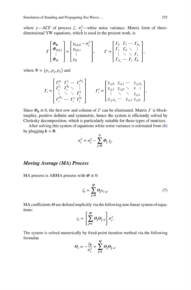
—white noise variance. Matrix form of threedimensional YW equations, which is used in the present work, is
í µí»¤
⎡
⎢
⎢
⎢
⎣
í µí»· í µí¿
í µí»· 0,0,1
⋮
í µí»· N
⎤
⎥
⎥
⎥
⎦
=
⎡
⎢
⎢
⎢
⎣
í µí»¾ 0,0,0 − í µí¼ 2
í µí¼
í µí»¾ 0,0,1
⋮
í µí»¾ N
⎤
⎥
⎥
⎥
⎦
,
í µí»¤ =
⎡
⎢
⎢
⎢
⎣
í µí»¤ 0 í µí»¤ 1 ⋯ í µí»¤ N 1
í µí»¤ 1 í µí»¤ 0 ⋱ ⋮
⋮ ⋱ ⋱ í µí»¤ 1
í µí»¤ N 1 ⋯ í µí»¤ 1 í µí»¤ 0
⎤
⎥
⎥
⎥
⎦
,
where N =
(
p 1 , p 2 , p 3
)
and
í µí»¤ i =
⎡
⎢
⎢
⎢
⎢
⎣
í µí»¤
0
i
í µí»¤
1
i
⋯ í µí»¤
N 2
i
í µí»¤
1
i
í µí»¤
0
i
⋱ ⋮
⋮ ⋱ ⋱ í µí»¤
1
i
í µí»¤
N 2
i
⋯ í µí»¤
1
i
í µí»¤
0
i
⎤
⎥
⎥
⎥
⎥
⎦
í µí»¤
j
i
=
⎡
⎢
⎢
⎢
⎣
í µí»¾ i,j,0 í µí»¾ i,j,1 ⋯ í µí»¾ i,j,N 3
í µí»¾ i,j,1 í µí»¾ i,j,0 ⋱ x ⋮
⋮ ⋱ ⋱ í µí»¾ i,j,1
í µí»¾ i,j,N 3 ⋯ í µí»¾ i,j,1 í µí»¾ i,j,0
⎤
⎥
⎥
⎥
⎦
,
Since í µí»· í µí¿ ≡ 0, the first row and column of í µí»¤ can be eliminated. Matrix í µí»¤ is blocktoeplitz, positive definite and symmetric, hence the system is efficiently solved by
Cholesky decomposition, which is particularly suitable for these types of matrices.
After solving this system of equations white noise variance is estimated from (6)
by plugging k = í µí¿:
í µí¼
2
í µí¼
= í µí¼
2
í µí¼
−
N
∑
j=í µí¿
í µí»· j í µí»¾ j .
Moving Average (MA) Process
MA process is ARMA process with í µí»· ≡ 0:
í µí¼ i =
M
∑
j=í µí¿
í µí»© j í µí¼ i−j .
(7)
MA coefficients í µí»© are defined implicitly via the following non-linear system of equations:
í µí»¾ i =
[ M
∑
j=i
í µí»© j í µí»© j−i
]
í µí¼
2
í µí¼ .
The system is solved numerically by fixed-point iteration method via the following
formulae
í µí»© i = −
í µí»¾ í µí¿
í µí¼ 2
í µí¼
+
M
∑
j=i
í µí»© j í µí»© j−i .
255
where í µí»¾—ACF of process í µí¼ , í µí¼ 2
í µí¼
—white noise variance. Matrix form of threedimensional YW equations, which is used in the present work, is
í µí»¤
⎡
⎢
⎢
⎢
⎣
í µí»· í µí¿
í µí»· 0,0,1
⋮
í µí»· N
⎤
⎥
⎥
⎥
⎦
=
⎡
⎢
⎢
⎢
⎣
í µí»¾ 0,0,0 − í µí¼ 2
í µí¼
í µí»¾ 0,0,1
⋮
í µí»¾ N
⎤
⎥
⎥
⎥
⎦
,
í µí»¤ =
⎡
⎢
⎢
⎢
⎣
í µí»¤ 0 í µí»¤ 1 ⋯ í µí»¤ N 1
í µí»¤ 1 í µí»¤ 0 ⋱ ⋮
⋮ ⋱ ⋱ í µí»¤ 1
í µí»¤ N 1 ⋯ í µí»¤ 1 í µí»¤ 0
⎤
⎥
⎥
⎥
⎦
,
where N =
(
p 1 , p 2 , p 3
)
and
í µí»¤ i =
⎡
⎢
⎢
⎢
⎢
⎣
í µí»¤
0
i
í µí»¤
1
i
⋯ í µí»¤
N 2
i
í µí»¤
1
i
í µí»¤
0
i
⋱ ⋮
⋮ ⋱ ⋱ í µí»¤
1
i
í µí»¤
N 2
i
⋯ í µí»¤
1
i
í µí»¤
0
i
⎤
⎥
⎥
⎥
⎥
⎦
í µí»¤
j
i
=
⎡
⎢
⎢
⎢
⎣
í µí»¾ i,j,0 í µí»¾ i,j,1 ⋯ í µí»¾ i,j,N 3
í µí»¾ i,j,1 í µí»¾ i,j,0 ⋱ x ⋮
⋮ ⋱ ⋱ í µí»¾ i,j,1
í µí»¾ i,j,N 3 ⋯ í µí»¾ i,j,1 í µí»¾ i,j,0
⎤
⎥
⎥
⎥
⎦
,
Since í µí»· í µí¿ ≡ 0, the first row and column of í µí»¤ can be eliminated. Matrix í µí»¤ is blocktoeplitz, positive definite and symmetric, hence the system is efficiently solved by
Cholesky decomposition, which is particularly suitable for these types of matrices.
After solving this system of equations white noise variance is estimated from (6)
by plugging k = í µí¿:
í µí¼
2
í µí¼
= í µí¼
2
í µí¼
−
N
∑
j=í µí¿
í µí»· j í µí»¾ j .
Moving Average (MA) Process
MA process is ARMA process with í µí»· ≡ 0:
í µí¼ i =
M
∑
j=í µí¿
í µí»© j í µí¼ i−j .
(7)
MA coefficients í µí»© are defined implicitly via the following non-linear system of equations:
í µí»¾ i =
[ M
∑
j=i
í µí»© j í µí»© j−i
]
í µí¼
2
í µí¼ .
The system is solved numerically by fixed-point iteration method via the following
formulae
í µí»© i = −
í µí»¾ í µí¿
í µí¼ 2
í µí¼
+
M
∑
j=i
í µí»© j í µí»© j−i .