

Simulation of Standing and Propagating Sea Waves . . .
253
í µí¼í µí¼
í µí¼x
|
|
|
|x,t
= −
1
√
1 + í µí»¼ 2
e
−I(x)
x
∫
0
í µí¼ ̇
í µí¼ ∕í µí¼z + í µí»¼ ̇
í µí»¼
√
1 + í µí»¼ 2
e
I(x) dx,
(3)
I(x) =
x
∫
0
í µí¼í µí»¼∕í µí¼z
1 + í µí»¼ 2 dx,
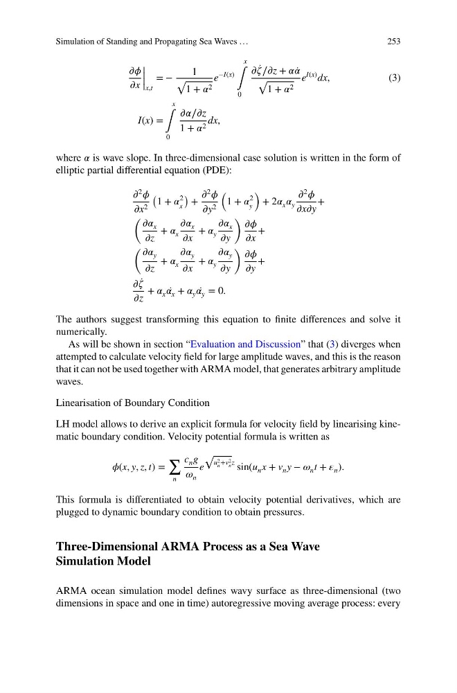
where í µí»¼ is wave slope. In three-dimensional case solution is written in the form of
elliptic partial differential equation (PDE):
í µí¼ 2 í µí¼
í µí¼x 2
(
1 + í µí»¼
2
x
) +
í µí¼ 2 í µí¼
í µí¼y 2
(
1 + í µí»¼
2
y
)
+ 2í µí»¼ x í µí»¼ y
í µí¼ 2 í µí¼
í µí¼xí µí¼y
+
( í µí¼í µí»¼ x
í µí¼z
+ í µí»¼ x
í µí¼í µí»¼ x
í µí¼x
+ í µí»¼ y
í µí¼í µí»¼ x
í µí¼y
) í µí¼í µí¼
í µí¼x
+
( í µí¼í µí»¼ y
í µí¼z
+ í µí»¼ x
í µí¼í µí»¼ y
í µí¼x
+ í µí»¼ y
í µí¼í µí»¼ y
í µí¼y
) í µí¼í µí¼
í µí¼y
+
í µí¼ ̇
í µí¼
í µí¼z
+ í µí»¼ x ̇
í µí»¼ x + í µí»¼ y ̇
í µí»¼ y = 0.
The authors suggest transforming this equation to finite differences and solve it
numerically.
As will be shown in section “Evaluation and Discussion” that (3) diverges when
attempted to calculate velocity field for large amplitude waves, and this is the reason
that it can not be used together with ARMA model, that generates arbitrary amplitude
waves.
Linearisation of Boundary Condition
LH model allows to derive an explicit formula for velocity field by linearising kinematic boundary condition. Velocity potential formula is written as
í µí¼(x, y, z, t) =
∑
n
c n g
í µí¼ n
e
√
u 2
n +v 2
n z sin(u n x + v n y − í µí¼ n t + í µí¼ n ).
This formula is differentiated to obtain velocity potential derivatives, which are
plugged to dynamic boundary condition to obtain pressures.
Three-Dimensional ARMA Process as a Sea Wave
Simulation Model
ARMA ocean simulation model defines wavy surface as three-dimensional (two
dimensions in space and one in time) autoregressive moving average process: every
253
í µí¼í µí¼
í µí¼x
|
|
|
|x,t
= −
1
√
1 + í µí»¼ 2
e
−I(x)
x
∫
0
í µí¼ ̇
í µí¼ ∕í µí¼z + í µí»¼ ̇
í µí»¼
√
1 + í µí»¼ 2
e
I(x) dx,
(3)
I(x) =
x
∫
0
í µí¼í µí»¼∕í µí¼z
1 + í µí»¼ 2 dx,
where í µí»¼ is wave slope. In three-dimensional case solution is written in the form of
elliptic partial differential equation (PDE):
í µí¼ 2 í µí¼
í µí¼x 2
(
1 + í µí»¼
2
x
) +
í µí¼ 2 í µí¼
í µí¼y 2
(
1 + í µí»¼
2
y
)
+ 2í µí»¼ x í µí»¼ y
í µí¼ 2 í µí¼
í µí¼xí µí¼y
+
( í µí¼í µí»¼ x
í µí¼z
+ í µí»¼ x
í µí¼í µí»¼ x
í µí¼x
+ í µí»¼ y
í µí¼í µí»¼ x
í µí¼y
) í µí¼í µí¼
í µí¼x
+
( í µí¼í µí»¼ y
í µí¼z
+ í µí»¼ x
í µí¼í µí»¼ y
í µí¼x
+ í µí»¼ y
í µí¼í µí»¼ y
í µí¼y
) í µí¼í µí¼
í µí¼y
+
í µí¼ ̇
í µí¼
í µí¼z
+ í µí»¼ x ̇
í µí»¼ x + í µí»¼ y ̇
í µí»¼ y = 0.
The authors suggest transforming this equation to finite differences and solve it
numerically.
As will be shown in section “Evaluation and Discussion” that (3) diverges when
attempted to calculate velocity field for large amplitude waves, and this is the reason
that it can not be used together with ARMA model, that generates arbitrary amplitude
waves.
Linearisation of Boundary Condition
LH model allows to derive an explicit formula for velocity field by linearising kinematic boundary condition. Velocity potential formula is written as
í µí¼(x, y, z, t) =
∑
n
c n g
í µí¼ n
e
√
u 2
n +v 2
n z sin(u n x + v n y − í µí¼ n t + í µí¼ n ).
This formula is differentiated to obtain velocity potential derivatives, which are
plugged to dynamic boundary condition to obtain pressures.
Three-Dimensional ARMA Process as a Sea Wave
Simulation Model
ARMA ocean simulation model defines wavy surface as three-dimensional (two
dimensions in space and one in time) autoregressive moving average process: every